Taxonomic Assignment
Overview
Teaching: 30 min
Exercises: 15 minQuestions
How can I know to which taxa my sequences belong?
Objectives
Understand how taxonomic assignment works.
Use Kraken to assign taxonomies to reads and contigs.
Visualize taxonomic assignations in graphics.
What is a taxonomic assignment?
A taxonomic assignment is a process of assigning an Operational Taxonomic Unit (OTU, that is, groups of related individuals) to sequences that can be reads or contigs. Sequences are compared against a database constructed using complete genomes. When a sequence finds a good enough match in the database, it is assigned to the corresponding OTU. The comparison can be made in different ways.
Strategies for taxonomic assignment
There are many programs for doing taxonomic mapping, and almost all of them follow one of the following strategies:
-
BLAST: Using BLAST or DIAMOND, these mappers search for the most likely hit for each sequence within a database of genomes (i.e., mapping). This strategy is slow.
-
Markers: They look for markers of a database made a priori in the sequences to be classified and assigned the taxonomy depending on the hits obtained.
-
K-mers: A genome database is broken into pieces of length k to be able to search for unique pieces by taxonomic group, from a lowest common ancestor (LCA), passing through phylum to species. Then, the algorithm breaks the query sequence (reads/contigs) into pieces of length k, looks for where these are placed within the tree and make the classification with the most probable position.
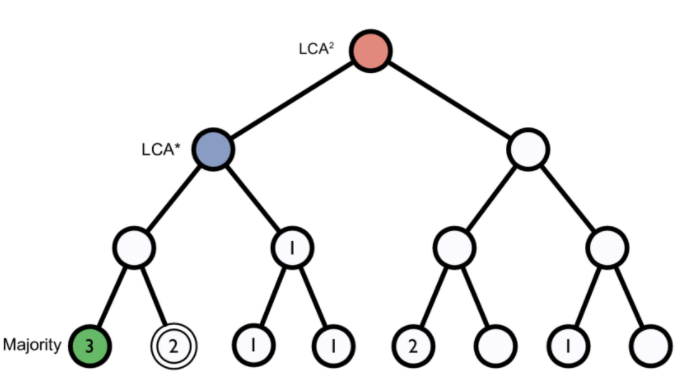 Figure 1. Lowest common ancestor assignment example.
Abundance bias
When you do the taxonomic assignment of metagenomes, a key result is the abundance of each taxon or OTU in your sample. The absolute abundance of a taxon is the number of sequences (reads or contigs, depending on what you did) assigned to it. Moreover, its relative abundance is the proportion of sequences assigned to it. It is essential to be aware of the many biases that can skew the abundances along the metagenomics workflow, shown in the figure, and that because of them, we may not be obtaining the actual abundance of the organisms in the sample.
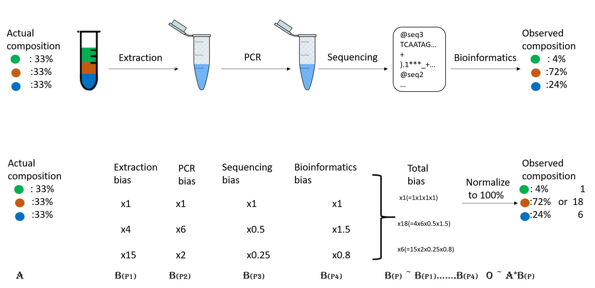 Figure 2. Abundance biases during a metagenomics protocol.
Discussion: Taxonomic level of assignment
What do you think is harder to assign, a species (like E. coli) or a phylum (like Proteobacteria)?
Using Kraken 2
Kraken 2 is the newest version of Kraken,
a taxonomic classification system using exact k-mer matches to achieve
high accuracy and fast classification speeds. kraken2 is already installed in the metagenomics
environment, let us have a look at kraken2 help.
$ kraken2 --help
Need to specify input filenames!
Usage: kraken2 [options] <filename(s)>

Options:
  --db NAME               Name for Kraken 2 DB
                          (default: none)
  --threads NUM           Number of threads (default: 1)
  --quick                 Quick operation (use first hit or hits)
  --unclassified-out FILENAME
                          Print unclassified sequences to filename
  --classified-out FILENAME
                          Print classified sequences to filename
  --output FILENAME       Print output to filename (default: stdout); "-" will
                          suppress normal output
  --confidence FLOAT      Confidence score threshold (default: 0.0); must be
                          in [0, 1].
  --minimum-base-quality NUM
                          Minimum base quality used in classification (def: 0,
                          only effective with FASTQ input).
  --report FILENAME       Print a report with aggregate counts/clade to file
  --use-mpa-style         With --report, format report output like Kraken 1's
                          kraken-mpa-report
  --report-zero-counts    With --report, report counts for ALL taxa, even if
                          counts are zero
  --report-minimizer-data With --report, report minimizer, and distinct minimizer
                          count information in addition to normal Kraken report
  --memory-mapping        Avoids loading database into RAM
  --paired                The filenames provided have paired-end reads
  --use-names             Print scientific names instead of just taxids
  --gzip-compressed       Input files are compressed with gzip
  --bzip2-compressed      Input files are compressed with bzip2
  --minimum-hit-groups NUM
                          Minimum number of hit groups (overlapping k-mers
                          sharing the same minimizer) needed to make a call
                          (default: 2)
  --help                  Print this message
  --version               Print version information

If none of the *-compressed flags are specified, and the filename provided
is a regular file, automatic format detection is attempted.
In the help, we can see that in addition to our input files, we also need a database to compare them. The database you use will determine the result you get for your data. Imagine you are searching for a recently discovered lineage that is not part of the available databases. Would you find it?
There are several databases compatible to be used with kraken2 in the taxonomical assignment process.
Unfortunately, even the smallest Kraken database Minikraken, which needs 8Gb of free RAM, is not small enough to be run by the machines we are using, so we will not be able to run kraken2. We can check our available RAM with free -hto be sure of this.
$ free -h
              total        used        free      shared  buff/cache   available
Mem:           3.9G        272M        3.3G         48M        251M        3.3G
Swap:            0B          0B          0B
Taxonomic assignment of metagenomic reads
As we have learned, taxonomic assignments can be attempted before the assembly.
In this case, we would use FASTQ files as inputs, which would be
JP4D_R1.trim.fastq.gz and JP4D_R2.trim.fastq.gz. And the outputs would be two files: the report
JP4D.report and the kraken file JP4D.kraken.
To run kraken2, we would use a command like this:
No need to run this
$ mkdir TAXONOMY_READS
$ kraken2 --db kraken-db --threads 8 --paired JP4D_R1.trim.fastq.gz JP4D_R2.trim.fastq.gz --output TAXONOMY_READS/JP4D.kraken --report TAXONOMY_READS/JP4D.report
Since we cannot run kraken2 here, we precomputed its results in a server, i.e., a more powerful machine.
In the server we ran kraken2 and obtainedJP4D-kraken.kraken and JP4D.report.
Let us look at the precomputed outputs of kraken2 for our JP4D reads.
head ~/dc_workshop/taxonomy/JP4D.kraken
U	MISEQ-LAB244-W7:156:000000000-A80CV:1:1101:19691:2037	0	250|251	0:216 |:| 0:217
U	MISEQ-LAB244-W7:156:000000000-A80CV:1:1101:14127:2052	0	250|238	0:216 |:| 0:204
U	MISEQ-LAB244-W7:156:000000000-A80CV:1:1101:14766:2063	0	251|251	0:217 |:| 0:217
C	MISEQ-LAB244-W7:156:000000000-A80CV:1:1101:15697:2078	2219696	250|120	0:28 350054:5 1224:2 0:1 2:5 0:77 2219696:5 0:93 |:| 379:4 0:82
U	MISEQ-LAB244-W7:156:000000000-A80CV:1:1101:15529:2080	0	250|149	0:216 |:| 0:115
U	MISEQ-LAB244-W7:156:000000000-A80CV:1:1101:14172:2086	0	251|250	0:217 |:| 0:216
U	MISEQ-LAB244-W7:156:000000000-A80CV:1:1101:17552:2088	0	251|249	0:217 |:| 0:215
U	MISEQ-LAB244-W7:156:000000000-A80CV:1:1101:14217:2104	0	251|227	0:217 |:| 0:193
C	MISEQ-LAB244-W7:156:000000000-A80CV:1:1101:15110:2108	2109625	136|169	0:51 31989:5 2109625:7 0:39 |:| 0:5 74033:2 31989:5 1077935:1 31989:7 0:7 60890:2 0:105 2109625:1
C	MISEQ-LAB244-W7:156:000000000-A80CV:1:1101:19558:2111	119045	251|133	0:18 1224:9 2:5 119045:4 0:181 |:| 0:99
This information may need to be clarified. Let us take out our cheatsheet to understand some of its components:
| Column example | Description |
|---|---|
| C | Classified or unclassified |
| MISEQ-LAB244-W7:156:000000000-A80CV:1:1101:15697:2078 | FASTA header of the sequence |
| 2219696 | Tax ID |
| 250:120 | Read length |
| 0:28 350054:5 1224:2 0:1 2:5 0:77 2219696:5 0:93 379:4 0:82 | kmers hit to a taxonomic ID e.g., tax ID 350054 has five hits, tax ID 1224 has two hits, etc. |
The Kraken file could be more readable. So let us look at the report file:
head ~/dc_workshop/taxonomy/JP4D.report
 78.13	587119	587119	U	0	unclassified
 21.87	164308	1166	R	1	root
 21.64	162584	0	R1	131567	  cellular organisms
 21.64	162584	3225	D	2	    Bacteria
 18.21	136871	3411	P	1224	      Proteobacteria
 14.21	106746	3663	C	28211	        Alphaproteobacteria
  7.71	57950	21	O	204455	          Rhodobacterales
  7.66	57527	6551	F	31989	            Rhodobacteraceae
  1.23	9235	420	G	1060	              Rhodobacter
  0.76	5733	4446	S	1063	                Rhodobacter sphaeroides
| Column example | Description |
|---|---|
| 78.13 | Percentage of reads covered by the clade rooted at this taxon |
| 587119 | Number of reads covered by the clade rooted at this taxon |
| 587119 | Number of reads assigned directly to this taxon |
| U | A rank code, indicating (U)nclassified, (D)omain, (K)ingdom, (P)hylum, (C)lass, (O)rder, (F)amily, (G)enus, or (S)pecies. All other ranks are simply ‘-‘. |
| 0 | NCBI taxonomy ID |
| unclassified | Indented scientific name |
Taxonomic assignment of the contigs of a MAG
We now have the taxonomic identity of the reads of the whole metagenome, but we need to know to which taxon our MAGs correspond. For this, we have to make the taxonomic assignment with their contigs instead of its reads because we do not have the reads corresponding to a MAG separated from the reads of the entire sample.
For this, the kraken2 is a little bit different; here, we can look at the command for the JP4D.001.fasta MAG:
No need to run this
$ mkdir TAXONOMY_MAG
$ kraken2 --db kraken-db --threads 12 -input JP4D.001.fasta --output TAXONOMY_MAG/JP4D.001.kraken --report TAXONOMY_MAG/JP4D.001.report
The results of this are pre-computed in the ~/dc_workshop/taxonomy/mags_taxonomy/ directory
$ cd ~/dc_workshop/taxonomy/mags_taxonomy
$ ls
JP4D.001.kraken
JP4D.001.report
more ~/dc_workshop/taxonomy/mags_taxonomy/JP4D.001.report
 50.96	955	955	U	0	unclassified
 49.04	919	1	R	1	root
 48.83	915	0	R1	131567	  cellular organisms
 48.83	915	16	D	2	    Bacteria
 44.40	832	52	P	1224	      Proteobacteria
 19.37	363	16	C	28216	        Betaproteobacteria
 16.22	304	17	O	80840	          Burkholderiales
  5.66	106	12	F	506	            Alcaligenaceae
  2.72	51	3	G	517	              Bordetella
  1.12	21	21	S	2163011	                Bordetella sp. HZ20
  .
  .
  .
Looking at the report, we can see that half of the contigs are unclassified and that a tiny proportion of contigs have been assigned an OTU. This result is weird because we expected only one genome in the bin.
To exemplify how a report of a complete and not contaminated MAG should look like this; let us look at the report of this MAG from another study:
100.00	108	0	R	1	root
100.00	108	0	R1	131567	  cellular organisms
100.00	108	0	D	2	    Bacteria
100.00	108	0	P	1224	      Proteobacteria
100.00	108	0	C	28211	        Alphaproteobacteria
100.00	108	0	O	356	          Rhizobiales
100.00	108	0	F	41294	            Bradyrhizobiaceae
100.00	108	0	G	374	              Bradyrhizobium
100.00	108	108	S	2057741	                Bradyrhizobium sp. SK17
Visualization of taxonomic assignment results
After we have the taxonomy assignation, what follows is some visualization of our results. Krona is a hierarchical data visualization software. Krona allows data to be explored with zooming and multi-layered pie charts and supports several bioinformatics tools and raw data formats. To use Krona in our results, let us first go into our taxonomy directory, which contains the pre-calculated Kraken outputs.
Krona
With Krona, we will explore the taxonomy of the JP4D.001 MAG.
$ cd ~/dc_workshop/taxonomy/mags_taxonomy
Krona is called with the ktImportTaxonomy command that needs an input and an output file.
In our case, we will create the input file with columns three and four from JP4D.001.kraken file.
$ cut -f2,3 JP4D.001.kraken > JP4D.001.krona.input
Now we call Krona in our JP4D.001.krona.input file and save results in JP4D.001.krona.out.html.
$ ktImportTaxonomy JP4D.001.krona.input -o JP4D.001.krona.out.html
Loading taxonomy...
Importing JP4D.001.krona.input...
   [ WARNING ]  The following taxonomy IDs were not found in the local database and were set to root
                (if they were recently added to NCBI, use updateTaxonomy.sh to update the local
                database): 1804984 2109625 2259134
And finally, open another terminal on your local computer, download the Krona output and open it on a browser.
$ scp dcuser@ec2-3-235-238-92.compute-1.amazonaws.com:~/dc_workshop/taxonomy/JP4D.001.krona.out.html .
You will see a page like this:
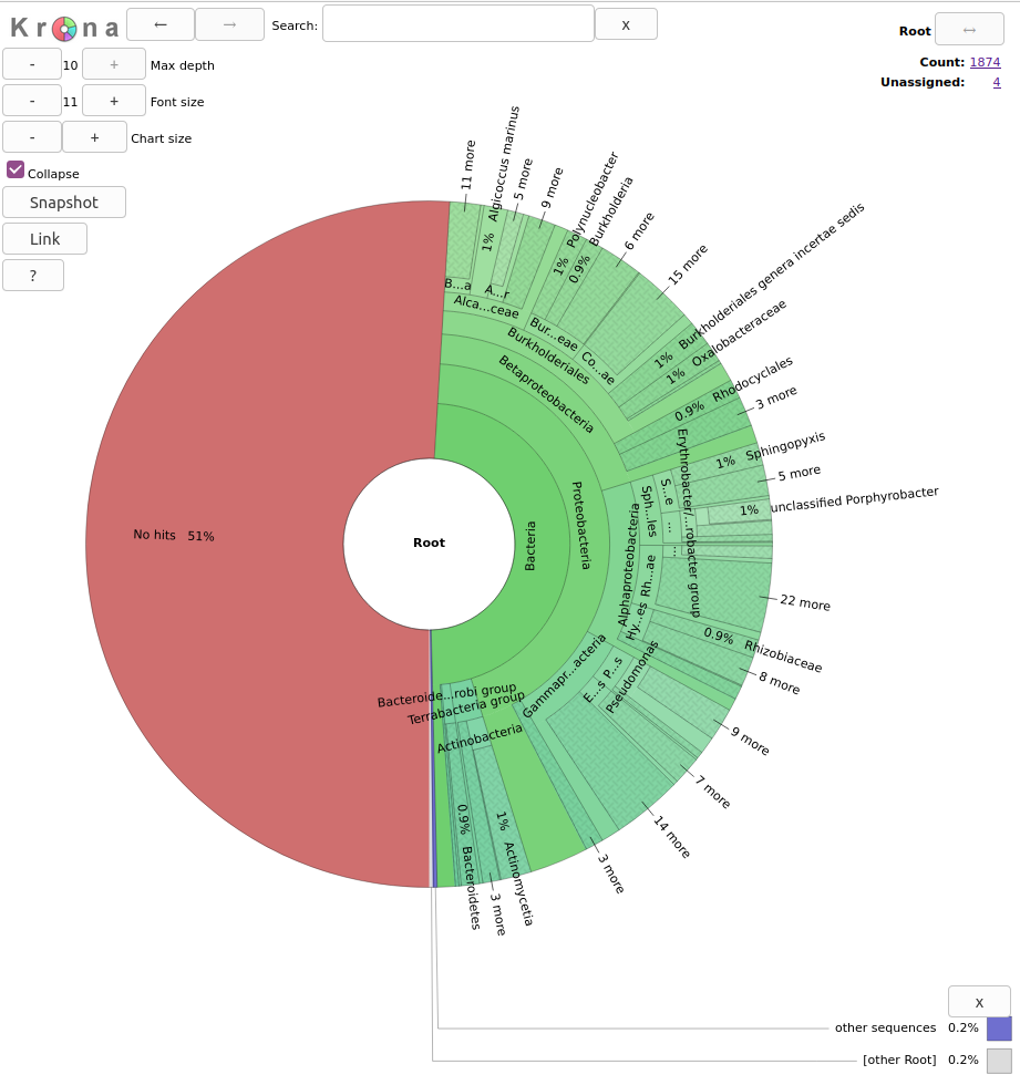
Exercise 1: Exploring Krona visualization
Try double-clicking on the pie chart segment representing Bacteria and see what happens. What percentage of bacteria is represented by the genus Paracoccus?
Hint: A search box is in the window’s top left corner.
Solution
2% of Bacteria corresponds to the genus Paracoccus in this sample. In the top right of the window, we see little pie charts that change whenever we change the visualization to expand certain taxa.
Pavian
Pavian is another visualization tool that allows comparison between multiple samples. Pavian should be locally installed and needs R and Shiny, but we can try the Pavian demo WebSite to visualize our results.
First, we need to download the files needed as inputs in Pavian; this time, we will visualize the
assignment of the reads of both samples:
JC1A.report and JP4D.report.
These files correspond to our Kraken reports. Again in our local
machine, let us use the scp command.
$ scp dcuser@ec2-3-235-238-92.compute-1.amazonaws.com:~/dc_workshop/taxonomy/*report .
We go to the Pavian demo WebSite, click on Browse, and choose our reports. You need to select both reports at the same time.
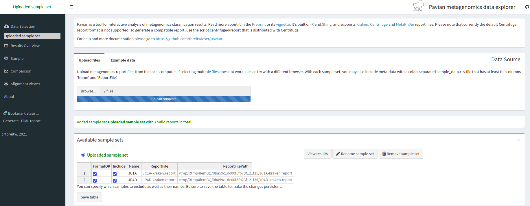
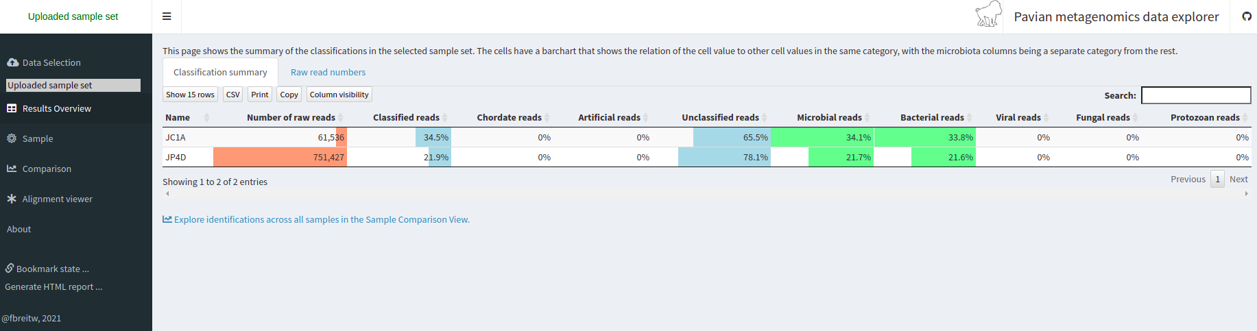
We click on the Results Overview tab.
We click on the Sample tab.
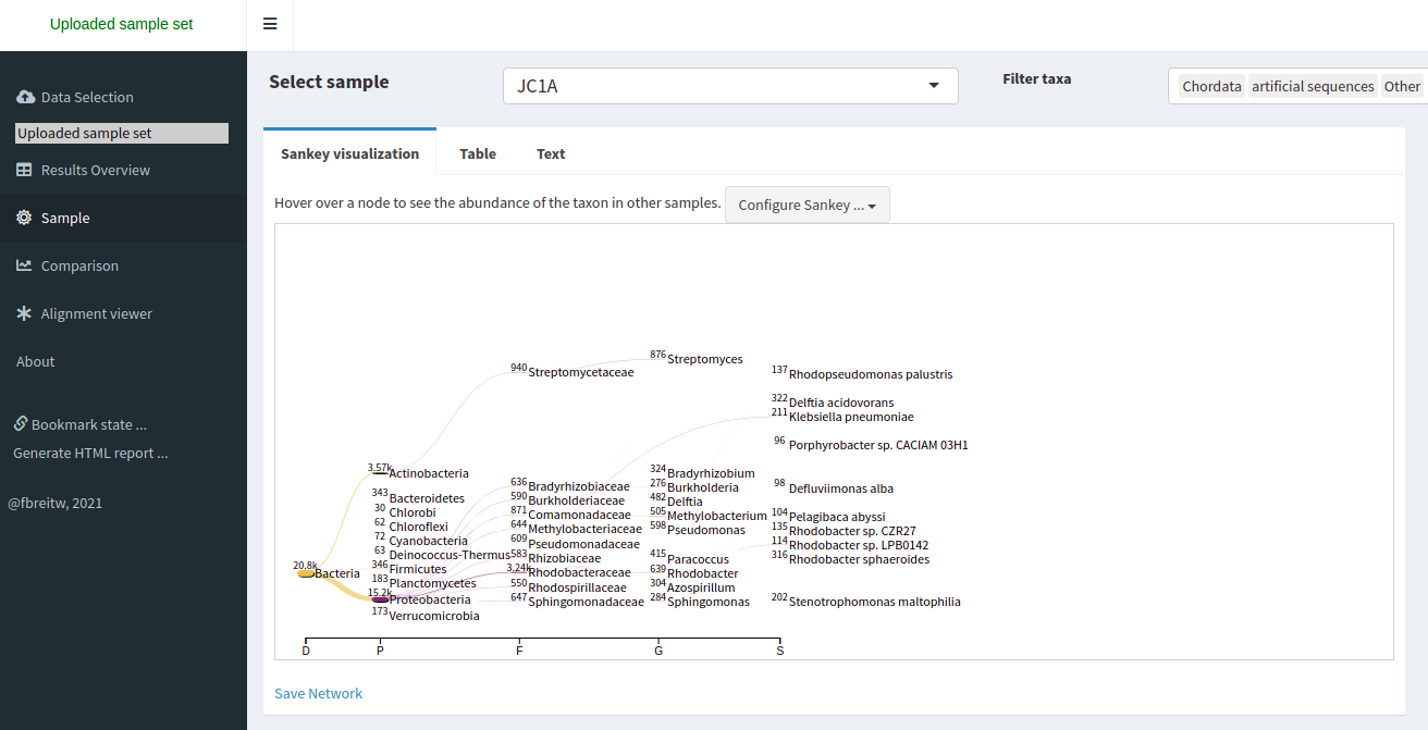
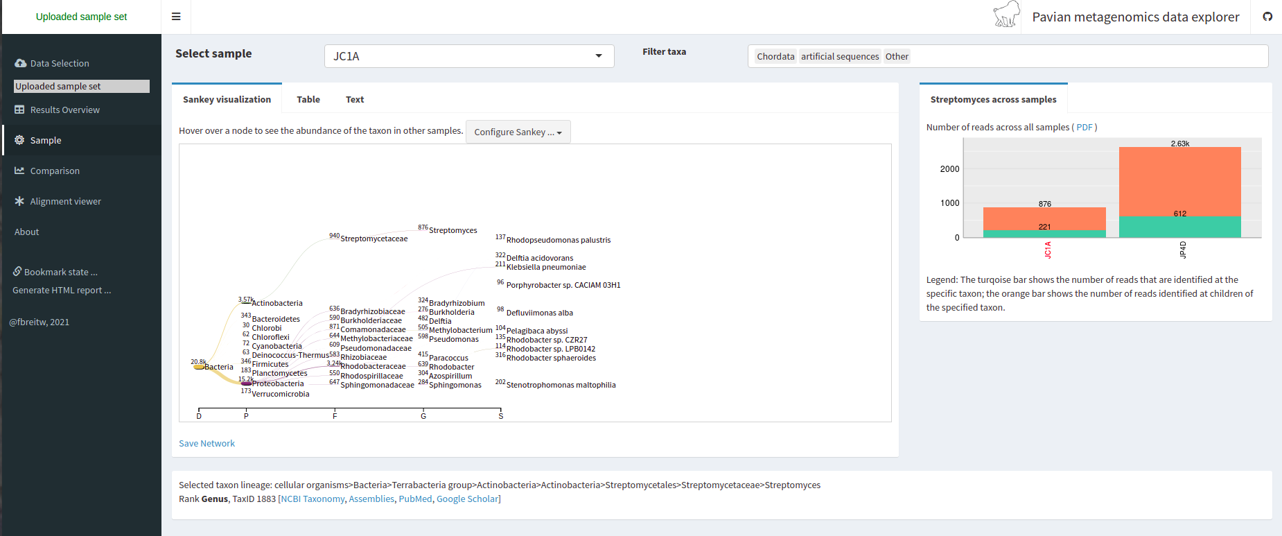
We can look at the abundance of a specific taxon by clicking on it.
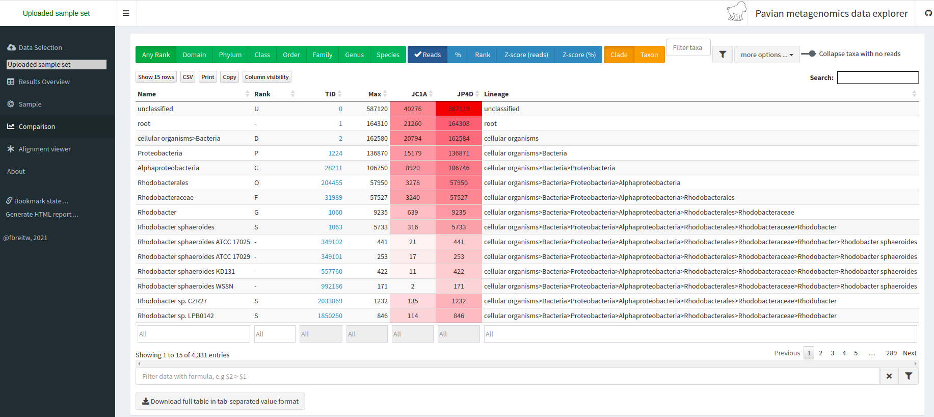
We can look at a comparison of both our samples in the Comparison tab.
Discussion: Unclassified reads
As you can see, a percentage of our data could not be assigned to belong to a specific OTU.
Which factors can affect the taxonomic assignation so that a read is unclassified?Solution
Unclassified reads can be the result of different factors that can go from sequencing errors to problems with the algorithm being used to generate the result. The widely used Next-generation sequencing (NGS) platforms, showed average error rate of 0.24±0.06% per base. Besides the sequencing error, we need to consider the status of the database being used to perform the taxonomic assignation.
All the characterized genomes obtained by different research groups are scattered in different repositories, pages, and banks in the cloud. Some are still unpublished. Incomplete databases can affect the performance of the taxonomic assignation. Imagine that the dominant OTU in your sample belongs to a lineage that has never been characterized and does not have a public genome available to be used as a template for the database. This possibility makes the assignation an impossible task and can promote the generation of false positives because the algorithm will assign a different identity to all those reads.
Key Points
A database with previously gathered knowledge (genomes) is needed for taxonomic assignment.
Taxonomic assignment can be done using Kraken.
Krona and Pavian are web-based tools to visualize the assigned taxa.