Summary and Setup
Python is rapidly emerging as the programming language of choice for data analysis in the atmosphere and ocean sciences. By consulting online tutorials and help pages, most researchers in this community are able to pick up the basic syntax and programming constructs (e.g. loops, lists and conditionals). This self-taught knowledge is sufficient to get work done, but it often involves spending hours to do things that should take minutes, reinventing a lot of wheels, and a nagging uncertainty at the end of it all regarding the reliability and reproducibility of the results. To help address these issues, these Data Carpentry lessons cover a suite of programming and data management best practices that aren’t so easy to glean from a quick Google search.
The skills covered in the lessons are taught in the context of a typical data analysis task: creating a command line program that plots the precipitation climatology for any given month, so that two different CMIP6 models (ACCESS-CM2 and ACCESS-ESM1-5) can be compared visually.
raster vs vector data
These lessons work with raster or “gridded” data that are stored as a uniform grid of values using the netCDF file format. This is the most common data format and file type in the atmosphere and ocean sciences; essentially all output from weather, climate and ocean models is gridded data stored as a series of netCDF files.
The other data type that atmosphere and ocean scientists tend to work with is geospatial vector data. In contrast to gridded raster data, these vector data are composed of discrete geometric locations (i.e. x, y values) that define the shape of a spatial point, line or polygon. They are not stored using the netCDF file format and are not covered in these lessons. Data Carpentry have separate lessons on working with geospatial vector data.
Prerequisites
Participants must have some familiarity with Python and the Unix
shell. They don’t need to be highly proficient, but a basic
understanding of Python syntax, beginner-level programming constructs
(e.g. loops and conditionals) and filesystem navigation using the shell
(e.g. the ls and cd commands) is required.
Citation
To cite these lessons, please refer to the following paper:
Irving D (2019). Python for atmosphere and ocean scientists. Journal of Open Source Education. 2(11), 37. doi:10.21105/jose.00037
Data
In preparation for these lessons, you will need to download the following two Python scripts and four netCDF files and place them in a new folder/directory:
- Make a new folder in your Desktop called
data-carpentry. - Download script_template.py and plot_precipitation_climatology.py and move them into that folder.
- Make a new folder in your
data_carpentryfolder calleddata. Download the following files and place them in that folder:
Software installation
In order to complete the lessons, you will need access to the following:
- The bash shell (the Z-shell is also fine, which is default on new Macs)
- A text editor
- Git
- Anaconda (which is a Python distribution)
If you don’t already have these installed, please follow The Carpentries software installation instructions. (You do not need to install R, which is also listed at that site.)
Troubeshooting
If you have any trouble with software installation, The Carpentries maintain a list of common issues on their Configuration Problems and Solutions wiki page.
Your workshop instructor may also ask that you install the python packages introduced in the first lesson ahead of time. You can do this via the command line or by using the Anaconda Navigator:
Installation of python packages: via the command line
(Windows users may need to open the Anaconda Prompt program and run
conda init bash to make conda available at the Bash
Shell.)
Step 1
Add the conda-forge channel:
Option 1 for Step 2 (recommended if you’re new to using Anaconda)
Install the packages in the base conda environment:
Option 2 for Step 2
Create a new environment called pyaos-lesson and install
the packages there:
You can activate this new environment as follows:
(Or source activate pyaos-lesson if that doesn’t
work.)
Type conda deactivate to exit that environment.
Installation of python packages: via the Anaconda Navigator
Once you’ve opened the Anaconda Navigator program (which can be found at the start menu on Windows), head to the “Environments” tab.
You can install the packages into the “base” environment (recommended
if you’re new to Anaconda) OR create a new environment called
pyaos-lesson by clicking the “create” button at the bottom
of the environment list before doing the following:
Step 1
Add the conda-forge channel. 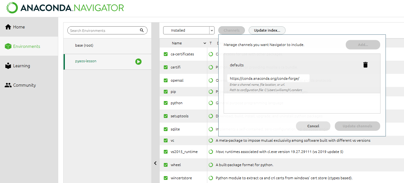
Step 2
Install the xarray, dask,
netCDF4, cartopy, cmocean and
cmdline_provenance packages one-by-one (click “apply” to
install once selected). If you’ve created a new environment, you’ll need
to install jupyter too. 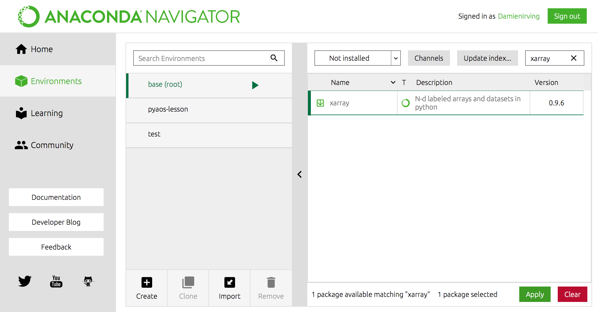
Software check
To check that everything is installed correctly, follow the instructions below.
Bash Shell
-
Linux: Open the Terminal program via the applications menu.
The default shell is usually Bash. If you aren’t sure what yours is,
type
echo $SHELL. If the shell listed is not bash, typebashand press Enter to access Bash. - Mac: Open the Applications Folder, and in Utilities select Terminal.
- Windows: Open the Git Bash program via the Windows start menu.
Git
- At the Bash Shell, type
git --version. You should see the version of your Git program listed.
Anaconda
- At the Bash Shell, type
python --version. You should see the version of your Python program listed, with a reference to Anaconda (i.e. the default Python program on your laptop needs to be the Anaconda installation of Python).