Functions

Last updated on 2024-07-25 | Edit this page

Overview

Questions

How can I define my own functions?

Objectives

Define a function that takes parameters.
Use docstrings to document functions.
Break our existing plotting code into a series of small, single-purpose functions.

In the previous lesson we created a plot of the ACCESS-CM2 historical precipitation climatology using the following commands:

PYTHON

import xarray as xr
import cartopy.crs as ccrs
import matplotlib.pyplot as plt
import numpy as np
import cmocean


accesscm2_pr_file = "data/pr_Amon_ACCESS-CM2_historical_r1i1p1f1_gn_201001-201412.nc"

ds = xr.open_dataset(accesscm2_pr_file)

clim = ds["pr"].groupby("time.season").mean("time", keep_attrs=True)

clim.data = clim.data * 86400
clim.attrs['units'] = "mm/day"

fig = plt.figure(figsize=[12,5])
ax = fig.add_subplot(111, projection=ccrs.PlateCarree(central_longitude=180))
clim.sel(season="JJA").plot.contourf(
    ax=ax,
    levels=np.arange(0, 13.5, 1.5),
    extend="max",
    transform=ccrs.PlateCarree(),
    cbar_kwargs={"label": clim.units},
    cmap=cmocean.cm.haline_r,
)
ax.coastlines()

model = ds.attrs["source_id"]
title = f"{model} precipitation climatology (JJA)"
plt.title(title)

plt.show()

If we wanted to create a similar plot for a different model and/or different month, we could cut and paste the code and edit accordingly. The problem with that (common) approach is that it increases the chances of a making a mistake. If we manually updated the season to ‘DJF’ for the clim.sel(season= command but forgot to update it when calling plt.title, for instance, we’d have a mismatch between the data and title.

The cut and paste approach is also much more time consuming. If we think of a better way to create this plot in future (e.g. we might want to add gridlines using plt.gca().gridlines()), then we have to find and update every copy and pasted instance of the code.

A better approach is to put the code in a function. The code itself then remains untouched, and we simply call the function with different input arguments.

PYTHON

def plot_pr_climatology(pr_file, season, gridlines=False):
    """Plot the precipitation climatology.
    
    Args:
      pr_file (str): Precipitation data file
      season (str): Season (3 letter abbreviation, e.g. JJA)
      gridlines (bool): Select whether to plot gridlines
    
    """

    ds = xr.open_dataset(pr_file)

    clim = ds["pr"].groupby("time.season").mean("time", keep_attrs=True)

    clim.data = clim.data * 86400
    clim.attrs["units"] = "mm/day"

    fig = plt.figure(figsize=[12,5])
    ax = fig.add_subplot(111, projection=ccrs.PlateCarree(central_longitude=180))
    clim.sel(season=season).plot.contourf(
        ax=ax,
        levels=np.arange(0, 13.5, 1.5),
        extend="max",
        transform=ccrs.PlateCarree(),
        cbar_kwargs={"label": clim.units},
        cmap=cmocean.cm.haline_r,
    )
    ax.coastlines()
    if gridlines:
        plt.gca().gridlines()
    
    model = ds.attrs["source_id"]
    title = f"{model} precipitation climatology ({season})"
    plt.title(title)

The docstring allows us to have good documentation for our function:

PYTHON

help(plot_pr_climatology)

OUTPUT

Help on function plot_pr_climatology in module __main__:

plot_pr_climatology(pr_file, season, gridlines=False)
    Plot the precipitation climatology.

    Args:
      pr_file (str): Precipitation data file
      season (str): Season (3 letter abbreviation, e.g. JJA)
      gridlines (bool): Select whether to plot gridlines

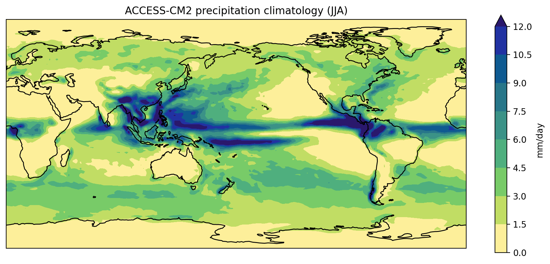
We can now use this function to create exactly the same plot as before:

PYTHON

plot_pr_climatology("data/pr_Amon_ACCESS-CM2_historical_r1i1p1f1_gn_201001-201412.nc", "JJA")
plt.show()

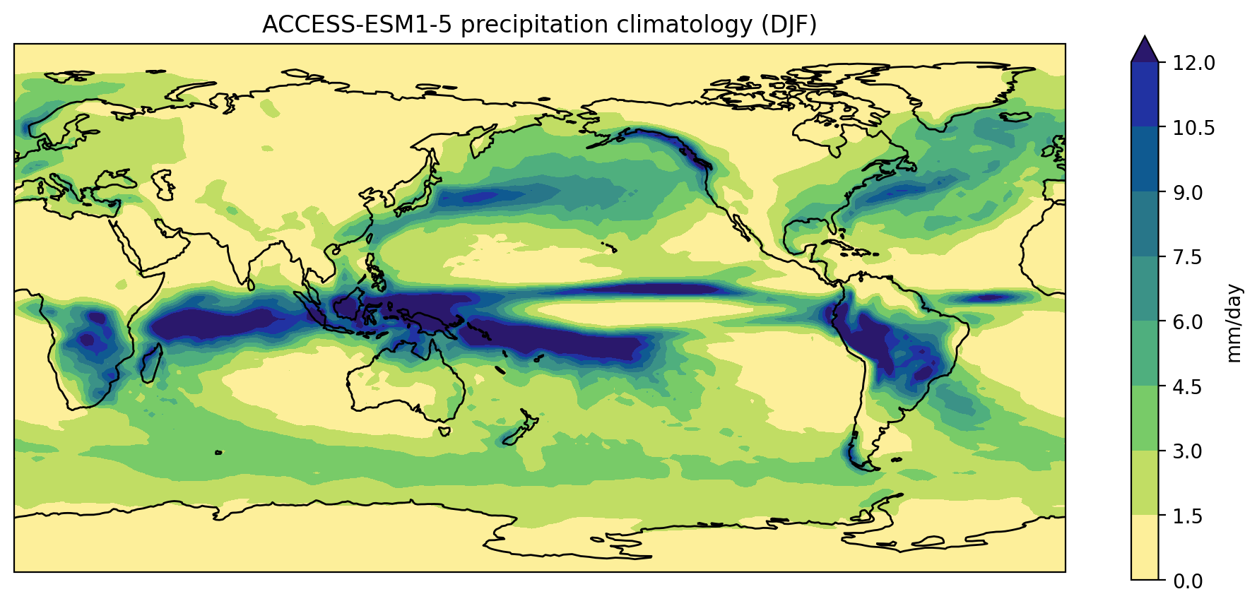
Plot a different model and season:

PYTHON

plot_pr_climatology("data/pr_Amon_ACCESS-ESM1-5_historical_r1i1p1f1_gn_201001-201412.nc", "DJF")
plt.show()

Or use the optional gridlines input argument to change the default behaviour of the function (keyword arguments are usually used for options that the user will only want to change occasionally):

PYTHON

plot_pr_climatology(
    "data/pr_Amon_ACCESS-ESM1-5_historical_r1i1p1f1_gn_201001-201412.nc",
    "DJF",
    gridlines=True,
)
plt.show()

Short functions

Our plot_pr_climatology function works, but at 16 lines of code it’s starting to get a little long. In general, people can only fit around 7-12 pieces of information in their short term memory. The readability of your code can therefore be greatly enhanced by keeping your functions short and sharp. The speed at which people can analyse their data is usually limited by the time it takes to read/understand/edit their code (as opposed to the time it takes the code to actually run), so the frequent use of short, well documented functions can dramatically speed up your data science.

Cut and paste the plot_pr_climatology function (defined in the notes above) into your own notebook and try running it with different input arguments.
Break the contents of plot_pr_climatology down into a series of smaller functions, such that it reads as follows:

PYTHON

def plot_pr_climatology(pr_file, season, gridlines=False):
    """Plot the precipitation climatology.

    Args:
      pr_file (str): Precipitation data file
      season (str): Season (3 letter abbreviation, e.g. JJA)
      gridlines (bool): Select whether to plot gridlines

    """

    ds = xr.open_dataset(pr_file)
    clim = ds["pr"].groupby("time.season").mean("time", keep_attrs=True)
    clim = convert_pr_units(clim)
    create_plot(clim, ds.attrs["source_id"], season, gridlines=gridlines)
    plt.show()

In other words, you’ll need to define new convert_pr_units and create_plot functions using code from the existing plot_pr_climatology function.

Show me the solution

PYTHON

def convert_pr_units(da):
    """Convert kg m-2 s-1 to mm day-1.
   
    Args:
      da (xarray.DataArray): Precipitation data
   
    """
   
    da.data = da.data * 86400
    da.attrs['units'] = "mm/day"
   
    return da


def create_plot(clim, model, season, gridlines=False):
    """Plot the precipitation climatology.
   
    Args:
      clim (xarray.DataArray): Precipitation climatology data
      model (str) : Name of the climate model
      season (str): Season 
   
    Kwargs:  
      gridlines (bool): Select whether to plot gridlines    
   
    """
       
    fig = plt.figure(figsize=[12,5])
    ax = fig.add_subplot(111, projection=ccrs.PlateCarree(central_longitude=180))
    clim.sel(season=season).plot.contourf(
        ax=ax,
        levels=np.arange(0, 13.5, 1.5),
        extend="max",
        transform=ccrs.PlateCarree(),
        cbar_kwargs={"label": clim.units},
        cmap=cmocean.cm.haline_r,
    )
    ax.coastlines()
    if gridlines:
        plt.gca().gridlines()
   
    title = f"{model} precipitation climatology ({season})"
    plt.title(title)


def plot_pr_climatology(pr_file, season, gridlines=False):
    """Plot the precipitation climatology.

    Args:
      pr_file (str): Precipitation data file
      season (str): Season (3 letter abbreviation, e.g. JJA)
      gridlines (bool): Select whether to plot gridlines

    """

    ds = xr.open_dataset(pr_file)
    clim = ds["pr"].groupby("time.season").mean("time", keep_attrs=True)
    clim = convert_pr_units(clim)
    create_plot(clim, ds.attrs["source_id"], season, gridlines=gridlines)
    plt.show()

Writing your own modules

We’ve used functions to avoid code duplication in this particular notebook/script, but what if we wanted to convert precipitation units from kg m-2 s-1 to mm/day in a different notebook/script?

To avoid cutting and pasting from this notebook/script to another, the solution would be to place the convert_pr_units function in a separate script full of similar functions.

For instance, we could put all our unit conversion functions in a script called unit_conversion.py. When we want to convert precipitation units (in any script or notebook we’re working on), we can simply import that “module” and use the convert_pr_units function:

PYTHON

import unit_conversion
clim.data = unit_conversion.convert_pr_units(clim.data)

No copy and paste required!

Key Points

Define a function using def name(...params...).
The body of a function must be indented.
Call a function using name(...values...).
Use help(thing) to view help for something.
Put docstrings in functions to provide help for that function.
Specify default values for parameters when defining a function using name=value in the parameter list.
The readability of your code can be greatly enhanced by using numerous short functions.
Write (and import) modules to avoid code duplication.