Content from Package management
Last updated on 2024-07-25 | Edit this page
Estimated time: 30 minutes
Overview
Questions
- What are the main Python libraries used in atmosphere and ocean science?
- How do I install and manage all the Python libraries that I want to use?
- How do I interact with Python?
Objectives
- Identify the main Python libraries used in atmosphere and ocean science and the relationships between them.
- Explain the advantages of Anaconda over other Python distributions.
- Extend the number of packages available via conda using conda-forge.
- Create a conda environment with the libraries needed for these lessons.
- Open a Jupyter Notebook ready for use in these lessons
The PyAOS stack
Before we jump in and start analysing our netCDF precipitation data files, we need to consider what Python libraries are best suited to the task.
For reading, writing and analysing data stored in the netCDF file format, atmosphere and ocean scientists will typically do most of their work with either the xarray or iris libraries. These libraries are built on top of more generic data science libraries like numpy and matplotlib, to make the types of analysis we do faster and more efficient. To learn more about the PyAOS “stack” shown in the diagram below (i.e. the collection of libraries that are typically used for data analysis and visualisation in the atmosphere and ocean sciences), check out the overview of the PyAOS stack at the PyAOS community site.

Python distributions for data science
Now that we’ve identified the Python libraries we might want to use, how do we go about installing them?
Our first impulse might be to use the Python package installer (pip), but it really only works for libraries written in pure Python. This is a major limitation for the data science community, because many scientific Python libraries have C and/or Fortran dependencies. To spare people the pain of installing these dependencies, a number of scientific Python “distributions” have been released over the years. These come with the most popular data science libraries and their dependencies pre-installed, and some also come with a package manager to assist with installing additional libraries that weren’t pre-installed. Today the most popular distribution for data science is Anaconda, which comes with a package (and environment) manager called conda.
Introducing conda
According to the latest documentation,
Anaconda comes with over 300 of the most widely used data science
libraries (and their dependencies) pre-installed. In addition, there are
several thousand more libraries available via the Anaconda Public
Repository, which can be installed by running the
conda install command the Bash Shell or Anaconda Prompt
(Windows only). It is also possible to install packages using the
Anaconda Navigator graphical user interface.
conda in the shell on windows
If you’re on a Windows machine and the conda command
isn’t available at the Bash Shell, you’ll need to open the Anaconda
Prompt program (via the Windows start menu) and run the command
conda init bash (this only needs to be done once). After
that, your Bash Shell will be configured to use conda going
forward.
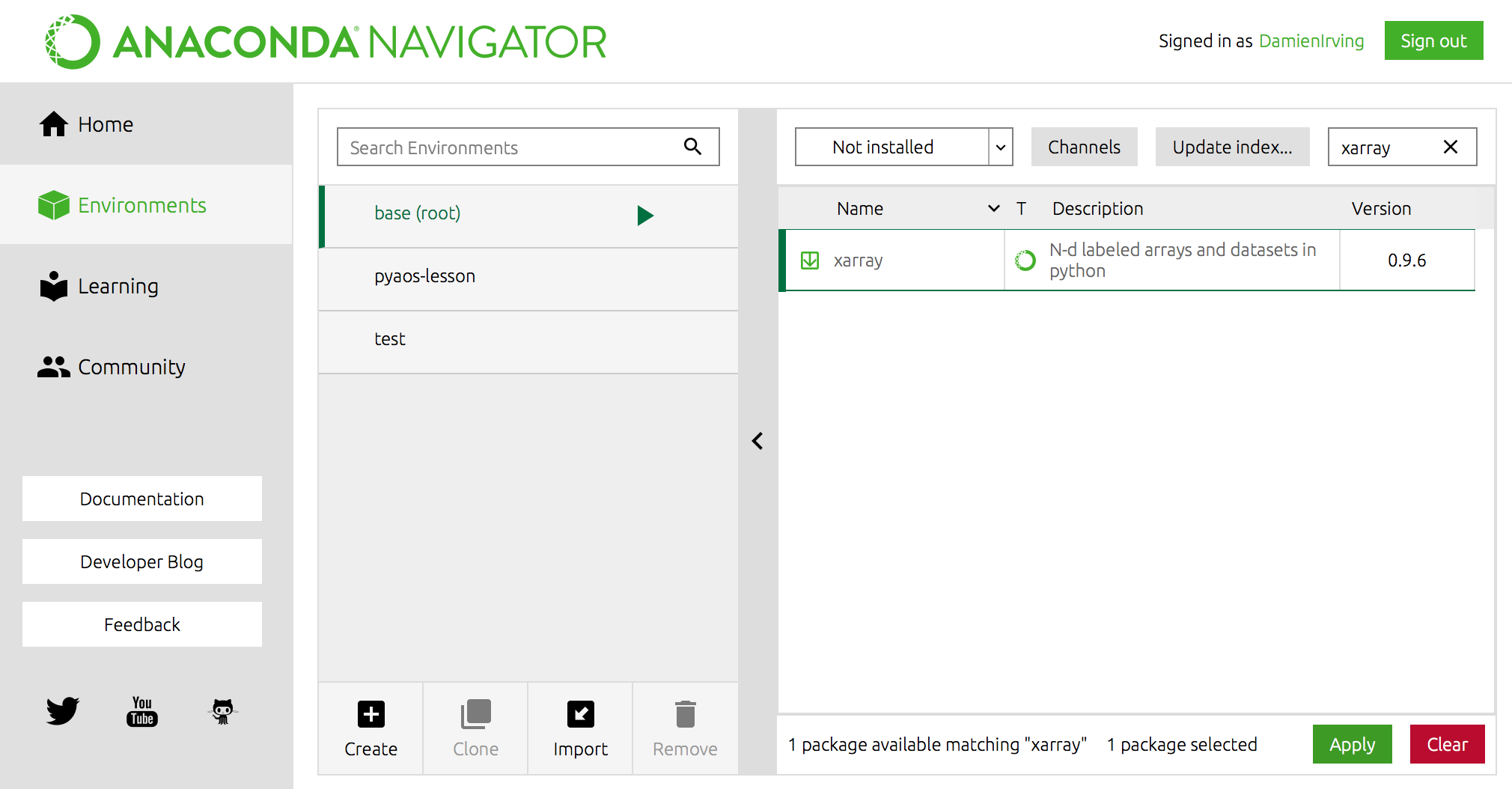
For instance, the popular xarray library could be
installed using the following command,
(Use conda search -f {package_name} to find out if a
package you want is available.)
OR using Anaconda Navigator:
Miniconda
If you don’t want to install the entire Anaconda distribution, you can install Miniconda instead. It essentially comes with conda and nothing else.
Advanced conda
For a relatively small/niche field of research like atmosphere and ocean science, one of the most important features that Anaconda provides is the Anaconda Cloud website, where the community can contribute conda installation packages. This is critical because many of our libraries have a small user base, which means they’ll never make it into the Anaconda Public Repository.
You can search Anaconda Cloud to find the command needed to install
the package. For instance, here is the search result for the
iris package:
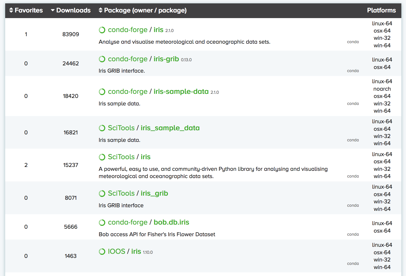
As you can see, there are often multiple versions of the same package
up on Anaconda Cloud. To try and address this duplication problem, conda-forge has been launched, which
aims to be a central repository that contains just a single (working)
version of each package on Anaconda Cloud. You can therefore expand the
selection of packages available via conda install beyond
the chosen few thousand by adding the conda-forge channel:
OR
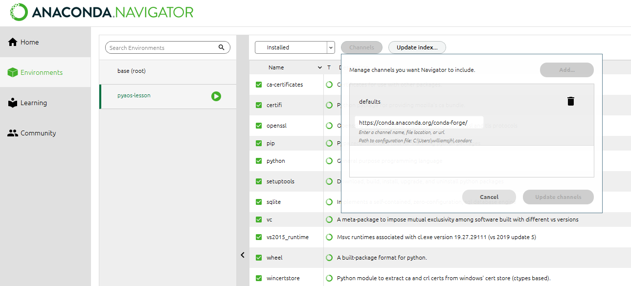
We recommend not adding any other third-party channels unless absolutely necessary, because mixing packages from multiple channels can cause headaches like binary incompatibilities.
Software installation for these lessons
For these particular lessons we will use xarray, but all
the same tasks could be performed with iris. We’ll also
install dask
(xarray uses this for parallel processing), netCDF4
(xarray requires this to read netCDF files), cartopy (to
help with geographic plot projections), cmocean (for
nice color palettes) and cmdline_provenance
(to keep track of our data processing steps). We don’t need to worry
about installing jupyter (we will be
using the jupyter notebook) because it already comes pre-installed with
Anaconda.
We could install these libraries from Anaconda Navigator (not shown) or using the Bash Shell or Anaconda Prompt (Windows):
If we then list all the libraries that we’ve got installed, we can
see that jupyter, dask, xarray,
netCDF4, cartopy, cmocean,
cmdline_provenance and their dependencies are now
there:
(This list can also be viewed in the environments tab of the Navigator.)
Creating separate environments
If you’ve got multiple data science projects on the go, installing all your packages in the same conda environment can get a little messy. (By default they are installed in the root/base environment.) It’s therefore common practice to create separate conda environments for the various projects you’re working on.
For instance, we could create an environment called
pyaos-lesson for this lesson. The process of creating a new
environment can be managed in the environments tab of the Anaconda
Navigator or via the following Bash Shell / Anaconda Prompt
commands:
BASH
$ conda create -n pyaos-lesson jupyter xarray dask netCDF4 cartopy cmocean cmdline_provenance
$ conda activate pyaos-lesson
(it’s conda deactivate to exit)
Notice that in this case we had to include jupyter in the list of packages to install. When you create a brand new conda environment, it doesn’t automatically come with the pre-installed packages that are in the base environment.
You can have lots of different environments,
OUTPUT
# conda environments:
#
base                  *  /anaconda3
pyaos-lesson             /anaconda3/envs/pyaos-lesson
test                     /anaconda3/envs/test
the details of which can be exported to a YAML configuration file:
OUTPUT
name: pyaos-lesson
channels:
  - conda-forge
  - defaults
dependencies:
  - cartopy=0.16.0=py36h81b52dc_1
  - certifi=2018.4.16=py36_0
  - cftime=1.0.1=py36h7eb728f_0
  - ...
Other people (or you on a different computer) can then re-create that exact environment using the YAML file:
The ease with which others can recreate your environment (on any operating system) is a huge breakthough for reproducible research.
To delete the environment:
Interacting with Python
Now that we know which Python libraries we want to use and how to install them, we need to decide how we want to interact with Python.
The most simple way to use Python is to type code directly into the interpreter. This can be accessed from the bash shell:
$ python
Python 3.7.1 (default, Dec 14 2018, 13:28:58)
[Clang 4.0.1 (tags/RELEASE_401/final)] :: Anaconda, Inc. on darwin
Type "help", "copyright", "credits" or "license" for more information.
>>> print("hello world")
hello world
>>> exit()
$
The >>> prompt indicates that you are now
talking to the Python interpreter.
A more powerful alternative to the default Python interpreter is IPython (Interactive Python). The online documentation outlines all the special features that come with IPython, but as an example, it lets you execute bash shell commands without having to exit the IPython interpreter:
$ ipython
Python 3.7.1 (default, Dec 14 2018, 13:28:58)
Type 'copyright', 'credits' or 'license' for more information
IPython 7.2.0 -- An enhanced Interactive Python. Type '?' for help.

In [1]: print("hello world")
hello world

In [2]: ls
data/                              script_template.py
plot_precipitation_climatology.py

In [3]: exit
$
(The IPython interpreter can also be accessed via the Anaconda Navigator by running the QtConsole.)
While entering commands to the Python or IPython interpreter line-by-line is great for quickly testing something, it’s clearly impractical for developing longer bodies of code and/or interactively exploring data. As such, Python users tend to do most of their code development and data exploration using either an Integrated Development Environment (IDE) or Jupyter Notebook:
- Two of the most common IDEs are Spyder and PyCharm (the former comes with Anaconda) and will look very familiar to anyone who has used MATLAB or R-Studio.
- Jupyter Notebooks run in your web browser and allow users to create and share documents that contain live code, equations, visualizations and narrative text.
We are going to use the Jupyter Notebook to explore our precipitation
data (and the plotting functionality of xarray) in the next few lessons.
A notebook can be launched from our data-carpentry
directory using the Bash Shell:
(The & allows you to come back and use the bash
shell without closing your notebook first.)
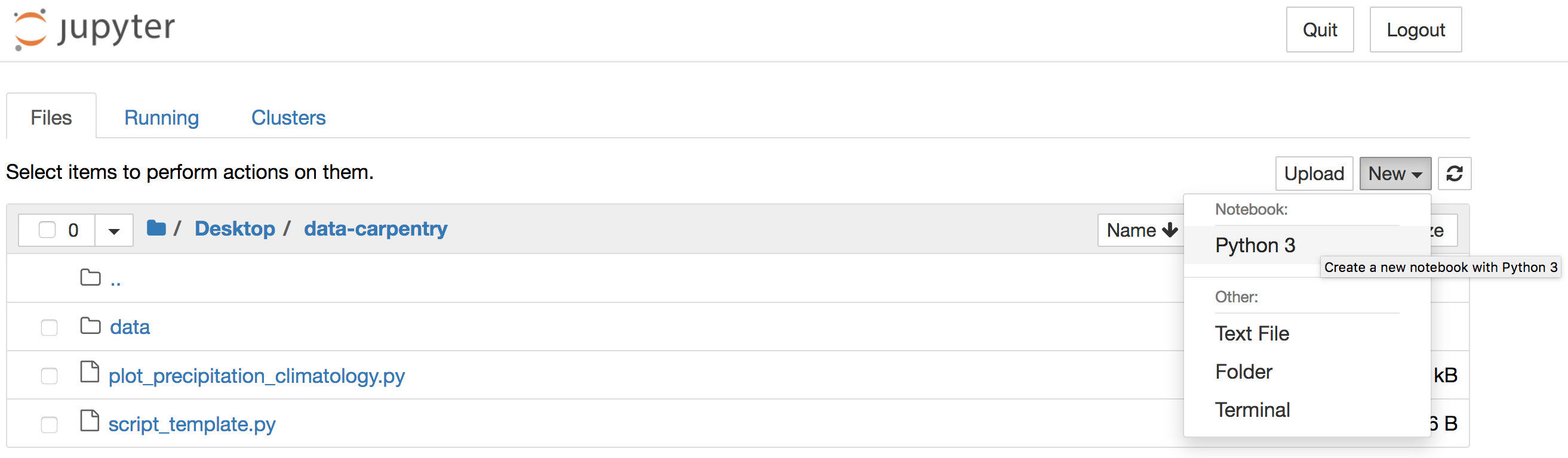
Alternatively, you can launch Jupyter Notebook from the Anaconda
Navigator and navigate to the data-carpentry directory
before creating a new Python 3 notebook:
JupyterLab
If you like Jupyter Notebooks you might want to try JupyterLab, which combines the Jupyter Notebook with many of the features common to an IDE.
Install the Python libraries required for this lesson
If you haven’t already done so, go ahead and install the
xarray, dask, netCDF4,
cartopy, cmocean and
cmdline_provenance packages using either the Anaconda
Navigator or Bash Shell.
Remember that you’ll need to add the conda-forge channel first.
(You may like to create a separate pyaos-lesson conda
environment, but this is not necessary to complete the lessons. If you
create a new environment rather than using the base environment, you’ll
need to install jupyter too.)
The software installation instructions explain how to install the Python libraries using the Bash Shell or Anaconda Navigator.
Launch a Jupyer Notebook
In preparation for the next lesson, open a new Jupyter Notebook
in your data-carpentry directory by
entering jupyter notebook & at the Bash Shell or by
clicking the Jupyter Notebook launch button in the Anaconda
Navigator.
If you use the Navigator, the Jupyter interface will open in a new
tab of your default web browser. Use that interface to navigate to the
data-carpentry directory that you created specifically for
these lessons before clicking to create a new Python 3 notebook:
Once your notebook is open, import xarray,
catropy, matplotlib and numpy
using the following Python commands:
PYTHON
import xarray as xr
import cartopy.crs as ccrs
import matplotlib.pyplot as plt
import numpy as np
(Hint: Hold down the shift and return keys to execute a code cell in a Jupyter Notebook.)
Key Points
- xarray and iris are the core Python libraries used in the atmosphere and ocean sciences.
- Use conda to install and manage your Python environments.
Content from Data processing and visualisation
Last updated on 2024-07-25 | Edit this page
Estimated time: 60 minutes
Overview
Questions
- How can I create a quick plot of my CMIP data?
Objectives
- Import the xarray library and use the functions it contains.
- Convert precipitation units to mm/day.
- Calculate and plot the precipitation climatology.
- Use the cmocean library to find colormaps designed for ocean science.
As a first step towards making a visual comparison of the ACCESS-CM2 and ACCESS-ESM1-5 historical precipitation climatology, we are going to create a quick plot of the ACCESS-CM2 data.
We will need a number of the libraries introduced in the previous lesson.
PYTHON
import xarray as xr
import cartopy.crs as ccrs
import matplotlib.pyplot as plt
import numpy as np
Since geographic data files can often be very large, when we first open our data file in xarray it simply loads the metadata associated with the file (this is known as “lazy loading”). We can then view summary information about the contents of the file before deciding whether we’d like to load some or all of the data into memory.
OUTPUT
<xarray.Dataset>
Dimensions:    (bnds: 2, lat: 144, lon: 192, time: 60)
Coordinates:
  * time       (time) datetime64[ns] 2010-01-16T12:00:00 ... 2014-12-16T12:00:00
  * lon        (lon) float64 0.9375 2.812 4.688 6.562 ... 355.3 357.2 359.1
  * lat        (lat) float64 -89.38 -88.12 -86.88 -85.62 ... 86.88 88.12 89.38
Dimensions without coordinates: bnds
Data variables:
    time_bnds  (time, bnds) datetime64[ns] ...
    lon_bnds   (lon, bnds) float64 ...
    lat_bnds   (lat, bnds) float64 ...
    pr         (time, lat, lon) float32 ...
Attributes:
    CDI:                    Climate Data Interface version 1.9.8 (https://mpi...
    source:                 ACCESS-CM2 (2019): \naerosol: UKCA-GLOMAP-mode\na...
    institution:            CSIRO (Commonwealth Scientific and Industrial Res...
    Conventions:            CF-1.7 CMIP-6.2
    activity_id:            CMIP
    branch_method:          standard
    branch_time_in_child:   0.0
    branch_time_in_parent:  0.0
    creation_date:          2019-11-08T08:26:37Z
    data_specs_version:     01.00.30
    experiment:             all-forcing simulation of the recent past
    experiment_id:          historical
    external_variables:     areacella
    forcing_index:          1
    frequency:              mon
    further_info_url:       https://furtherinfo.es-doc.org/CMIP6.CSIRO-ARCCSS...
    grid:                   native atmosphere N96 grid (144x192 latxlon)
    grid_label:             gn
    initialization_index:   1
    institution_id:         CSIRO-ARCCSS
    mip_era:                CMIP6
    nominal_resolution:     250 km
    notes:                  Exp: CM2-historical; Local ID: bj594; Variable: p...
    parent_activity_id:     CMIP
    parent_experiment_id:   piControl
    parent_mip_era:         CMIP6
    parent_source_id:       ACCESS-CM2
    parent_time_units:      days since 0950-01-01
    parent_variant_label:   r1i1p1f1
    physics_index:          1
    product:                model-output
    realization_index:      1
    realm:                  atmos
    run_variant:            forcing: GHG, Oz, SA, Sl, Vl, BC, OC, (GHG = CO2,...
    source_id:              ACCESS-CM2
    source_type:            AOGCM
    sub_experiment:         none
    sub_experiment_id:      none
    table_id:               Amon
    table_info:             Creation Date:(30 April 2019) MD5:e14f55f257cceaf...
    title:                  ACCESS-CM2 output prepared for CMIP6
    variable_id:            pr
    variant_label:          r1i1p1f1
    version:                v20191108
    cmor_version:           3.4.0
    tracking_id:            hdl:21.14100/b4dd0f13-6073-4d10-b4e6-7d7a4401e37d
    license:                CMIP6 model data produced by CSIRO is licensed un...
    CDO:                    Climate Data Operators version 1.9.8 (https://mpi...
    history:                Tue Jan 12 14:50:25 2021: ncatted -O -a history,p...
    NCO:                    netCDF Operators version 4.9.2 (Homepage = http:/...
We can see that our ds object is an
xarray.Dataset, which when printed shows all the metadata
associated with our netCDF data file.
In this case, we are interested in the precipitation variable contained within that xarray Dataset:
OUTPUT
<xarray.DataArray 'pr' (time: 60, lat: 144, lon: 192)>
[1658880 values with dtype=float32]
Coordinates:
  * time     (time) datetime64[ns] 2010-01-16T12:00:00 ... 2014-12-16T12:00:00
  * lon      (lon) float64 0.9375 2.812 4.688 6.562 ... 353.4 355.3 357.2 359.1
  * lat      (lat) float64 -89.38 -88.12 -86.88 -85.62 ... 86.88 88.12 89.38
Attributes:
    standard_name:  precipitation_flux
    long_name:      Precipitation
    units:          kg m-2 s-1
    comment:        includes both liquid and solid phases
    cell_methods:   area: time: mean
    cell_measures:  area: areacella
We can actually use either the ds["pr"] or
ds.pr syntax to access the precipitation
xarray.DataArray.
To calculate the precipitation climatology, we can make use of the fact that xarray DataArrays have built in functionality for averaging over their dimensions.
OUTPUT
<xarray.DataArray 'pr' (lat: 144, lon: 192)>
array([[1.8461452e-06, 1.9054805e-06, 1.9228980e-06, ..., 1.9869783e-06,
        2.0026005e-06, 1.9683730e-06],
       [1.9064508e-06, 1.9021350e-06, 1.8931637e-06, ..., 1.9433096e-06,
        1.9182237e-06, 1.9072245e-06],
       [2.1003202e-06, 2.0477617e-06, 2.0348527e-06, ..., 2.2391034e-06,
        2.1970161e-06, 2.1641599e-06],
       ...,
       [7.5109556e-06, 7.4777777e-06, 7.4689174e-06, ..., 7.3359679e-06,
        7.3987890e-06, 7.3978440e-06],
       [7.1837171e-06, 7.1722038e-06, 7.1926393e-06, ..., 7.1552149e-06,
        7.1576678e-06, 7.1592167e-06],
       [7.0353467e-06, 7.0403985e-06, 7.0326828e-06, ..., 7.0392648e-06,
        7.0387587e-06, 7.0304386e-06]], dtype=float32)
Coordinates:
  * lon      (lon) float64 0.9375 2.812 4.688 6.562 ... 353.4 355.3 357.2 359.1
  * lat      (lat) float64 -89.38 -88.12 -86.88 -85.62 ... 86.88 88.12 89.38
Attributes:
    standard_name:  precipitation_flux
    long_name:      Precipitation
    units:          kg m-2 s-1
    comment:        includes both liquid and solid phases
    cell_methods:   area: time: mean
    cell_measures:  area: areacella
Now that we’ve calculated the climatology, we want to convert the units from kg m-2 s-1 to something that we are a little more familiar with like mm day-1.
To do this, consider that 1 kg of rain water spread over 1 m2 of surface is 1 mm in thickness and that there are 86400 seconds in one day. Therefore, 1 kg m-2 s-1 = 86400 mm day-1.
The data associated with our xarray DataArray is simply a numpy array,
OUTPUT
numpy.ndarrayso we can go ahead and multiply that array by 86400 and update the units attribute accordingly:
OUTPUT
<xarray.DataArray 'pr' (lat: 144, lon: 192)>
array([[0.15950695, 0.16463352, 0.16613839, ..., 0.17167493, 0.17302468,
        0.17006743],
       [0.16471735, 0.16434446, 0.16356934, ..., 0.16790195, 0.16573453,
        0.1647842 ],
       [0.18146767, 0.17692661, 0.17581128, ..., 0.19345854, 0.18982219,
        0.18698342],
       ...,
       [0.64894656, 0.64607999, 0.64531446, ..., 0.63382763, 0.63925537,
        0.63917372],
       [0.62067316, 0.61967841, 0.62144403, ..., 0.61821057, 0.6184225 ,
        0.61855632],
       [0.60785395, 0.60829043, 0.60762379, ..., 0.60819248, 0.60814875,
        0.6074299 ]])
Coordinates:
  * lon      (lon) float64 0.9375 2.812 4.688 6.562 ... 353.4 355.3 357.2 359.1
  * lat      (lat) float64 -89.38 -88.12 -86.88 -85.62 ... 86.88 88.12 89.38
Attributes:
    standard_name:  precipitation_flux
    long_name:      Precipitation
    units:          mm/day
    comment:        includes both liquid and solid phases
    cell_methods:   area: time: mean
    cell_measures:  area: areacella
We could now go ahead and plot our climatology using matplotlib, but
it would take many lines of code to extract all the latitude and
longitude information and to setup all the plot characteristics.
Recognising this burden, the xarray developers have built on top of
matplotlib.pyplot to make the visualisation of xarray
DataArrays much easier.
PYTHON
fig = plt.figure(figsize=[12,5])

ax = fig.add_subplot(111, projection=ccrs.PlateCarree(central_longitude=180))

clim.plot.contourf(
    ax=ax,
    levels=np.arange(0, 13.5, 1.5),
    extend="max",
    transform=ccrs.PlateCarree(),
    cbar_kwargs={"label": clim.units}
)
ax.coastlines()

plt.show()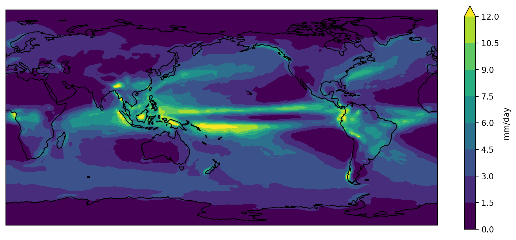
The default colorbar used by matplotlib is viridis. It
used to be jet, but that was changed in response to the #endtherainbow
campaign.
Putting all the code together (and reversing viridis so that wet is purple and dry is yellow)…
PYTHON
import xarray as xr
import cartopy.crs as ccrs
import matplotlib.pyplot as plt
import numpy as np


accesscm2_pr_file = "data/pr_Amon_ACCESS-CM2_historical_r1i1p1f1_gn_201001-201412.nc"

ds = xr.open_dataset(accesscm2_pr_file)

clim = ds["pr"].mean("time", keep_attrs=True)

clim.data = clim.data * 86400
clim.attrs["units"] = "mm/day"

fig = plt.figure(figsize=[12,5])
ax = fig.add_subplot(111, projection=ccrs.PlateCarree(central_longitude=180))
clim.plot.contourf(
    ax=ax,
    levels=np.arange(0, 13.5, 1.5),
    extend="max",
    transform=ccrs.PlateCarree(),
    cbar_kwargs={"label": clim.units},
    cmap="viridis_r",
)
ax.coastlines()
plt.show()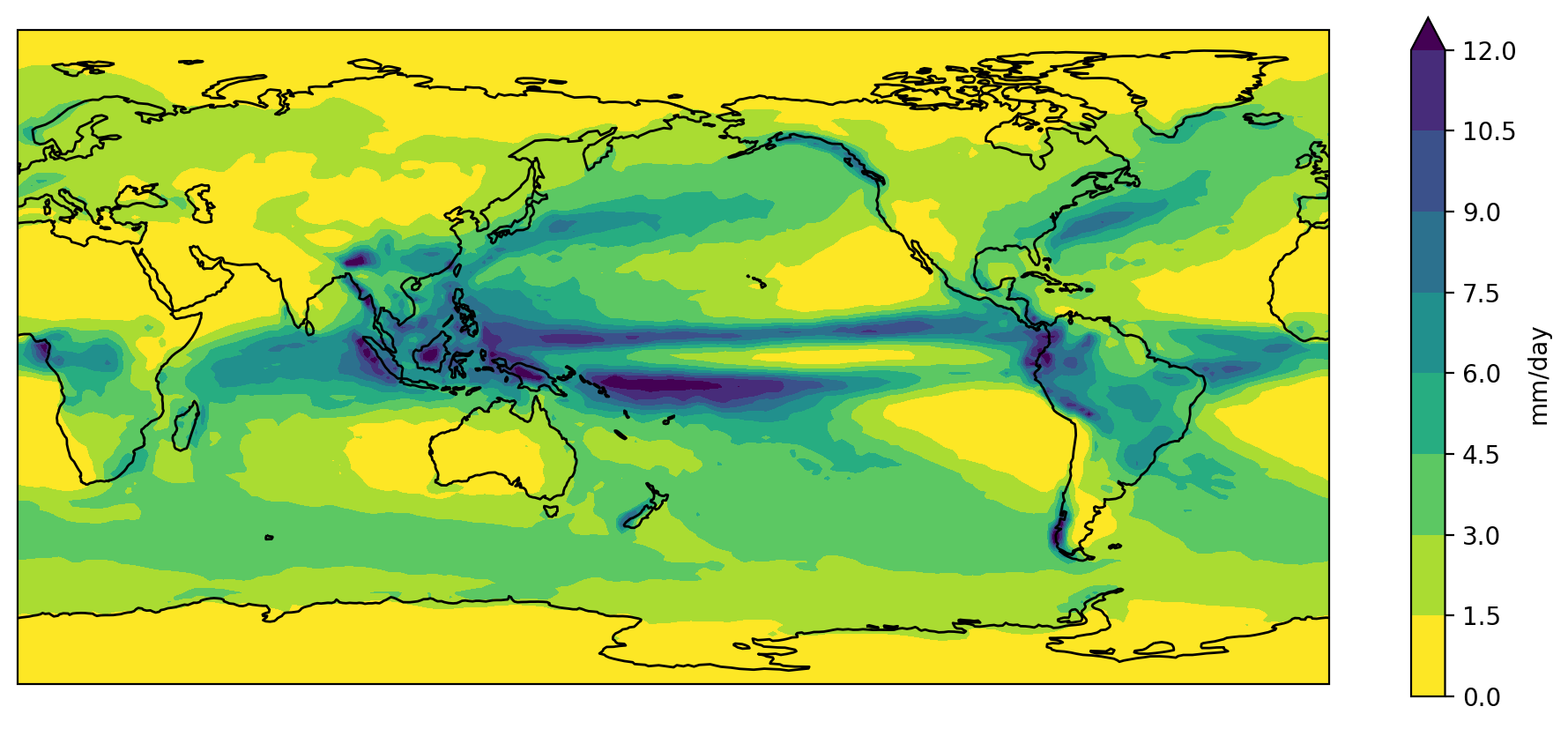
Color palette
Copy and paste the final slab of code above into your own Jupyter notebook.
The viridis color palette doesn’t seem quite right for rainfall. Change it to the “haline” cmocean palette used for ocean salinity data.
Season selection
Rather than plot the annual climatology, edit the code so that it plots the June-August (JJA) season.
(Hint: the groupby functionality can be used to group
all the data into seasons prior to averaging over the time axis)
Add a title
Add a title to the plot which gives the name of the model (taken from
the ds attributes) followed by the words “precipitation
climatology (JJA)”
Key Points
- Libraries such as xarray can make loading, processing and visualising netCDF data much easier.
- The cmocean library contains colormaps custom made for the ocean sciences.
Content from Functions
Last updated on 2024-07-25 | Edit this page
Estimated time: 40 minutes
Overview
Questions
- How can I define my own functions?
Objectives
- Define a function that takes parameters.
- Use docstrings to document functions.
- Break our existing plotting code into a series of small, single-purpose functions.
In the previous lesson we created a plot of the ACCESS-CM2 historical precipitation climatology using the following commands:
PYTHON
import xarray as xr
import cartopy.crs as ccrs
import matplotlib.pyplot as plt
import numpy as np
import cmocean
accesscm2_pr_file = "data/pr_Amon_ACCESS-CM2_historical_r1i1p1f1_gn_201001-201412.nc"
ds = xr.open_dataset(accesscm2_pr_file)
clim = ds["pr"].groupby("time.season").mean("time", keep_attrs=True)
clim.data = clim.data * 86400
clim.attrs['units'] = "mm/day"
fig = plt.figure(figsize=[12,5])
ax = fig.add_subplot(111, projection=ccrs.PlateCarree(central_longitude=180))
clim.sel(season="JJA").plot.contourf(
ax=ax,
levels=np.arange(0, 13.5, 1.5),
extend="max",
transform=ccrs.PlateCarree(),
cbar_kwargs={"label": clim.units},
cmap=cmocean.cm.haline_r,
)
ax.coastlines()
model = ds.attrs["source_id"]
title = f"{model} precipitation climatology (JJA)"
plt.title(title)
plt.show()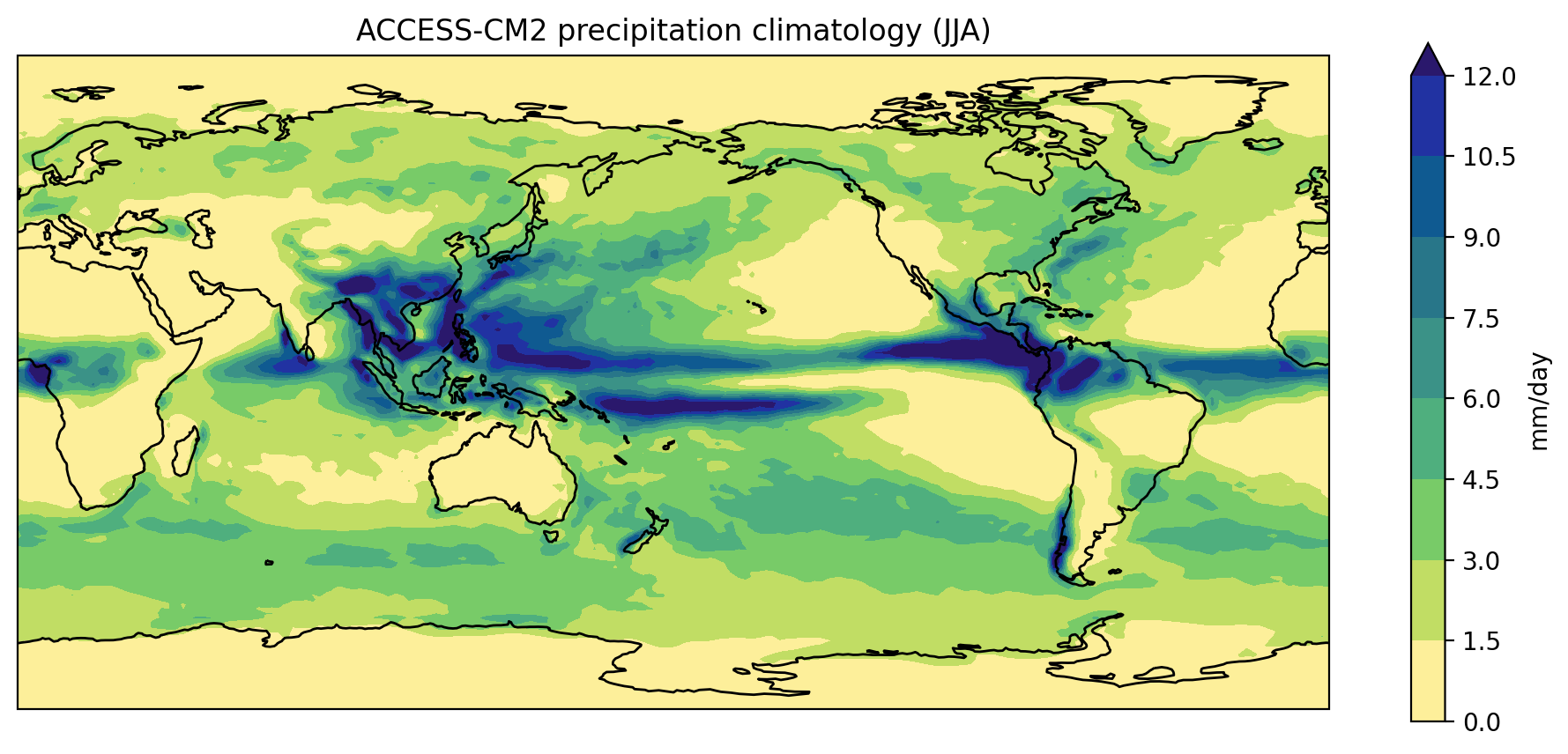
If we wanted to create a similar plot for a different model and/or
different month, we could cut and paste the code and edit accordingly.
The problem with that (common) approach is that it increases the chances
of a making a mistake. If we manually updated the season to ‘DJF’ for
the clim.sel(season= command but forgot to update it when
calling plt.title, for instance, we’d have a mismatch
between the data and title.
The cut and paste approach is also much more time consuming. If we
think of a better way to create this plot in future (e.g. we might want
to add gridlines using plt.gca().gridlines()), then we have
to find and update every copy and pasted instance of the code.
A better approach is to put the code in a function. The code itself then remains untouched, and we simply call the function with different input arguments.
PYTHON
def plot_pr_climatology(pr_file, season, gridlines=False):
    """Plot the precipitation climatology.

    Args:
      pr_file (str): Precipitation data file
      season (str): Season (3 letter abbreviation, e.g. JJA)
      gridlines (bool): Select whether to plot gridlines

    """

    ds = xr.open_dataset(pr_file)

    clim = ds["pr"].groupby("time.season").mean("time", keep_attrs=True)

    clim.data = clim.data * 86400
    clim.attrs["units"] = "mm/day"

    fig = plt.figure(figsize=[12,5])
    ax = fig.add_subplot(111, projection=ccrs.PlateCarree(central_longitude=180))
    clim.sel(season=season).plot.contourf(
        ax=ax,
        levels=np.arange(0, 13.5, 1.5),
        extend="max",
        transform=ccrs.PlateCarree(),
        cbar_kwargs={"label": clim.units},
        cmap=cmocean.cm.haline_r,
    )
    ax.coastlines()
    if gridlines:
        plt.gca().gridlines()

    model = ds.attrs["source_id"]
    title = f"{model} precipitation climatology ({season})"
    plt.title(title)
The docstring allows us to have good documentation for our function:
OUTPUT
Help on function plot_pr_climatology in module __main__:

plot_pr_climatology(pr_file, season, gridlines=False)
    Plot the precipitation climatology.

    Args:
      pr_file (str): Precipitation data file
      season (str): Season (3 letter abbreviation, e.g. JJA)
      gridlines (bool): Select whether to plot gridlines
We can now use this function to create exactly the same plot as before:
PYTHON
plot_pr_climatology("data/pr_Amon_ACCESS-CM2_historical_r1i1p1f1_gn_201001-201412.nc", "JJA")
plt.show()
Plot a different model and season:
PYTHON
plot_pr_climatology("data/pr_Amon_ACCESS-ESM1-5_historical_r1i1p1f1_gn_201001-201412.nc", "DJF")
plt.show()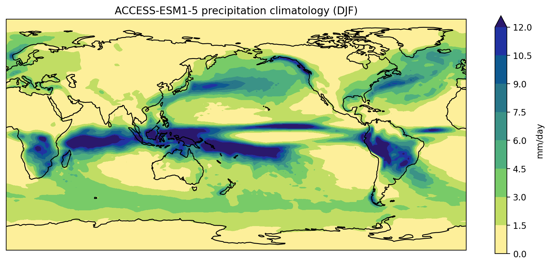
Or use the optional gridlines input argument to change
the default behaviour of the function (keyword arguments are usually
used for options that the user will only want to change
occasionally):
PYTHON
plot_pr_climatology(
    "data/pr_Amon_ACCESS-ESM1-5_historical_r1i1p1f1_gn_201001-201412.nc",
    "DJF",
    gridlines=True,
)
plt.show()
Short functions
Our plot_pr_climatology function works, but at 16 lines
of code it’s starting to get a little long. In general, people can only
fit around 7-12 pieces of information in their short term memory. The
readability of your code can therefore be greatly enhanced by keeping
your functions short and sharp. The speed at which people can analyse
their data is usually limited by the time it takes to
read/understand/edit their code (as opposed to the time it takes the
code to actually run), so the frequent use of short, well documented
functions can dramatically speed up your data science.
- Cut and paste the
plot_pr_climatologyfunction (defined in the notes above) into your own notebook and try running it with different input arguments. - Break the contents of
plot_pr_climatologydown into a series of smaller functions, such that it reads as follows:
PYTHON
def plot_pr_climatology(pr_file, season, gridlines=False):
    """Plot the precipitation climatology.

    Args:
      pr_file (str): Precipitation data file
      season (str): Season (3 letter abbreviation, e.g. JJA)
      gridlines (bool): Select whether to plot gridlines

    """

    ds = xr.open_dataset(pr_file)
    clim = ds["pr"].groupby("time.season").mean("time", keep_attrs=True)
    clim = convert_pr_units(clim)
    create_plot(clim, ds.attrs["source_id"], season, gridlines=gridlines)
    plt.show()
In other words, you’ll need to define new
convert_pr_units and create_plot functions
using code from the existing plot_pr_climatology
function.
PYTHON
def convert_pr_units(da):
    """Convert kg m-2 s-1 to mm day-1.

    Args:
      da (xarray.DataArray): Precipitation data

    """

    da.data = da.data * 86400
    da.attrs['units'] = "mm/day"

    return da


def create_plot(clim, model, season, gridlines=False):
    """Plot the precipitation climatology.

    Args:
      clim (xarray.DataArray): Precipitation climatology data
      model (str) : Name of the climate model
      season (str): Season

    Kwargs:
      gridlines (bool): Select whether to plot gridlines

    """

    fig = plt.figure(figsize=[12,5])
    ax = fig.add_subplot(111, projection=ccrs.PlateCarree(central_longitude=180))
    clim.sel(season=season).plot.contourf(
        ax=ax,
        levels=np.arange(0, 13.5, 1.5),
        extend="max",
        transform=ccrs.PlateCarree(),
        cbar_kwargs={"label": clim.units},
        cmap=cmocean.cm.haline_r,
    )
    ax.coastlines()
    if gridlines:
        plt.gca().gridlines()

    title = f"{model} precipitation climatology ({season})"
    plt.title(title)


def plot_pr_climatology(pr_file, season, gridlines=False):
    """Plot the precipitation climatology.

    Args:
      pr_file (str): Precipitation data file
      season (str): Season (3 letter abbreviation, e.g. JJA)
      gridlines (bool): Select whether to plot gridlines

    """

    ds = xr.open_dataset(pr_file)
    clim = ds["pr"].groupby("time.season").mean("time", keep_attrs=True)
    clim = convert_pr_units(clim)
    create_plot(clim, ds.attrs["source_id"], season, gridlines=gridlines)
    plt.show()
Writing your own modules
We’ve used functions to avoid code duplication in this particular notebook/script, but what if we wanted to convert precipitation units from kg m-2 s-1 to mm/day in a different notebook/script?
To avoid cutting and pasting from this notebook/script to another,
the solution would be to place the convert_pr_units
function in a separate script full of similar functions.
For instance, we could put all our unit conversion functions in a
script called unit_conversion.py. When we want to convert
precipitation units (in any script or notebook we’re working on), we can
simply import that “module” and use the convert_pr_units
function:
No copy and paste required!
Key Points
- Define a function using
def name(...params...). - The body of a function must be indented.
- Call a function using
name(...values...). - Use
help(thing)to view help for something. - Put docstrings in functions to provide help for that function.
- Specify default values for parameters when defining a function using
name=valuein the parameter list. - The readability of your code can be greatly enhanced by using numerous short functions.
- Write (and import) modules to avoid code duplication.
Content from Command line programs
Last updated on 2024-07-25 | Edit this page
Estimated time: 50 minutes
Overview
Questions
- How can I write my own command line programs?
Objectives
- Use the
argparselibrary to manage command-line arguments in a program. - Structure Python scripts according to a simple template.
We’ve arrived at the point where we have successfully defined the functions required to plot the precipitation data.
We could continue to execute these functions from the Jupyter notebook, but in most cases notebooks are simply used to try things out and/or take notes on a new data analysis task. Once you’ve scoped out the task (as we have for plotting the precipitation climatology), that code can be transferred to a Python script so that it can be executed at the command line. It’s likely that your data processing workflows will include command line utilities from the CDO and NCO projects in addition to Python code, so the command line is the natural place to manage your workflows (e.g. using shell scripts or make files).
In general, the first thing that gets added to any Python script is the following:
The reason we need these two lines of code is that running a Python script in bash is very similar to importing that file in Python. The biggest difference is that we don’t expect anything to happen when we import a file, whereas when running a script we expect to see some output (e.g. an output file, figure and/or some text printed to the screen).
The __name__ variable exists to handle these two
situations. When you import a Python file __name__ is set
to the name of that file (e.g. when importing script.py,
__name__ is script), but when running a script
in bash __name__ is always set to __main__.
The convention is to call the function that produces the output
main(), but you can call it whatever you like.
The next thing you’ll need is a library to parse the command line for input arguments. The most widely used option is argparse.
Putting those together, here’s a template for what most python command line programs look like:
PYTHON
import argparse

#
# All your functions (that will be called by main()) go here.
#

def main(inargs):
    """Run the program."""

    print("Input file: ", inargs.infile)
    print("Output file: ", inargs.outfile)


if __name__ == "__main__":

    description = "Print the input arguments to the screen."
    parser = argparse.ArgumentParser(description=description)

    parser.add_argument("infile", type=str, help="Input file name")
    parser.add_argument("outfile", type=str, help="Output file name")

    args = parser.parse_args()
    main(args)
By running script_template.py at the command line we’ll
see that argparse handles all the input arguments:
OUTPUT
Input file:  in.nc
Output file:  out.nc
It also generates help information for the user:
OUTPUT
usage: script_template.py [-h] infile outfile

Print the input arguments to the screen.

positional arguments:
  infile      Input file name
  outfile     Output file name

optional arguments:
  -h, --help  show this help message and exit
and issues errors when users give the program invalid arguments:
OUTPUT
usage: script_template.py [-h] infile outfile
script_template.py: error: the following arguments are required: outfile
Using this template as a starting point, we can add the functions we
developed previously to a script called
plot_precipitation_climatology.py.
PYTHON
import xarray as xr
import cartopy.crs as ccrs
import matplotlib.pyplot as plt
import numpy as np
import cmocean
import argparse


def convert_pr_units(da):
    """Convert kg m-2 s-1 to mm day-1.

    Args:
      da (xarray.DataArray): Precipitation data

    """

    da.data = darray.data * 86400
    da.attrs["units"] = "mm/day"

    return da


def create_plot(clim, model, season, gridlines=False):
    """Plot the precipitation climatology.

    Args:
      clim (xarray.DataArray): Precipitation climatology data
      model (str): Name of the climate model
      season (str): Season

    Kwargs:
      gridlines (bool): Select whether to plot gridlines

    """

    fig = plt.figure(figsize=[12,5])
    ax = fig.add_subplot(111, projection=ccrs.PlateCarree(central_longitude=180))
    clim.sel(season=season).plot.contourf(
        ax=ax,
        levels=np.arange(0, 13.5, 1.5),
        extend="max",
        transform=ccrs.PlateCarree(),
        cbar_kwargs={"label": clim.units},
        cmap=cmocean.cm.haline_r,
    )
    ax.coastlines()
    if gridlines:
        plt.gca().gridlines()

    title = f"{model} precipitation climatology ({season})"
    plt.title(title)


def main(inargs):
    """Run the program."""

    ds = xr.open_dataset(inargs.pr_file)

    clim = ds["pr"].groupby("time.season").mean("time", keep_attrs=True)
    clim = convert_pr_units(clim)

    create_plot(clim, ds.attrs["source_id"], inargs.season)
    plt.savefig(
        inargs.output_file,
        dpi=200,
        bbox_inches="tight",
        facecolor="white",
    )


if __name__ == "__main__":
    description='Plot the precipitation climatology.'
    parser = argparse.ArgumentParser(description=description)

    parser.add_argument("pr_file", type=str, help="Precipitation data file")
    parser.add_argument("season", type=str, help="Season to plot")
    parser.add_argument("output_file", type=str, help="Output file name")

    args = parser.parse_args()

    main(args)
… and then run it at the command line:
BASH
$ python plot_precipitation_climatology.py data/pr_Amon_ACCESS-CM2_historical_r1i1p1f1_gn_201001-201412.nc MAM pr_Amon_ACCESS-CM2_historical_r1i1p1f1_gn_201001-201412-MAM-clim.pngChoices
For this series of challenges, you are required to make improvements
to the plot_precipitation_climatology.py script that you
downloaded earlier from the setup tab at the top of the page.
For the first improvement, edit the line of code that defines the
season command line argument
(parser.add_argument("season", type=str, help="Season to plot"))
so that it only allows the user to input a valid three letter
abbreviation (i.e. ["DJF", "MAM", "JJA", "SON"]).
(Hint: Read about the choices keyword argument at the argparse
tutorial.)
Gridlines
Add an optional command line argument that allows the user to add gridlines to the plot.
(Hint: Read about the action="store_true" keyword
argument at the argparse
tutorial.)
Make the following additions to
plot_precipitation_climatology.py (code omitted from this
abbreviated version of the script is denoted ...):
Colorbar levels
Add an optional command line argument that allows the user to specify the tick levels used in the colourbar
(Hint: You’ll need to use the nargs='*' keyword
argument.)
Make the following additions to
plot_precipitation_climatology.py (code omitted from this
abbreviated version of the script is denoted ...):
PYTHON
...

def create_plot(clim, model_name, season, gridlines=False, levels=None):
    """Plot the precipitation climatology.
      ...
      Kwargs:
        gridlines (bool): Select whether to plot gridlines
        levels (list): Tick marks on the colorbar

    """

    if not levels:
        levels = np.arange(0, 13.5, 1.5)

    ...

    clim.sel(season=season).plot.contourf(
        ax=ax,
        ...,
    )

...

def main(inargs):

    ...

    create_plot(
        clim,
        ds.attrs["source_id"],
        inargs.season,
        gridlines=inargs.gridlines,
        levels=inargs.cbar_levels,
    )

...

if __name__ == "__main__":

    ...

    parser.add_argument(
        "--cbar_levels",
        type=float,
        nargs="*",
        default=None,
        help="list of levels / tick marks to appear on the colorbar",
    )

...
Free time
Add any other options you’d like for customising the plot (e.g. title, axis labels, figure size).
plot_precipitation_climatology.py
At the conclusion of this lesson your
plot_precipitation_climatology.py script should look
something like the following:
PYTHON
import xarray as xr
import cartopy.crs as ccrs
import matplotlib.pyplot as plt
import numpy as np
import cmocean
import argparse


def convert_pr_units(da):
    """Convert kg m-2 s-1 to mm day-1.

    Args:
      da (xarray.DataArray): Precipitation data

    """

    da.data = darray.data * 86400
    da.attrs["units"] = "mm/day"

    return da


def create_plot(clim, model, season, gridlines=False, levels=None):
    """Plot the precipitation climatology.

    Args:
      clim (xarray.DataArray): Precipitation climatology data
      model (str): Name of the climate model
      season (str): Season

    Kwargs:
      gridlines (bool): Select whether to plot gridlines
      levels (list): Tick marks on the colorbar

    """

    if not levels:
        levels = np.arange(0, 13.5, 1.5)

    fig = plt.figure(figsize=[12,5])
    ax = fig.add_subplot(111, projection=ccrs.PlateCarree(central_longitude=180))
    clim.sel(season=season).plot.contourf(
        ax=ax,
        levels=levels,
        extend="max",
        transform=ccrs.PlateCarree(),
        cbar_kwargs={"label": clim.units},
        cmap=cmocean.cm.haline_r,
    )
    ax.coastlines()
    if gridlines:
        plt.gca().gridlines()

    title = f"{model} precipitation climatology ({season})"
    plt.title(title)


def main(inargs):
    """Run the program."""

    ds = xr.open_dataset(inargs.pr_file)

    clim = ds["pr"].groupby("time.season").mean("time", keep_attrs=True)
    clim = convert_pr_units(clim)

    create_plot(
        clim,
        ds.attrs["source_id"],
        inargs.season,
        gridlines=inargs.gridlines,
        levels=inargs.cbar_levels,
    )
    plt.savefig(
        inargs.output_file,
        dpi=200,
        bbox_inches="tight",
        facecolor="white",
    )


if __name__ == "__main__":
    description = "Plot the precipitation climatology."
    parser = argparse.ArgumentParser(description=description)

    parser.add_argument("pr_file", type=str, help="Precipitation data file")
    parser.add_argument("season", type=str, help="Season to plot")
    parser.add_argument("output_file", type=str, help="Output file name")

    parser.add_argument(
        "--gridlines",
        action="store_true",
        default=False,
        help="Include gridlines on the plot",
    )
    parser.add_argument(
        "--cbar_levels",
        type=float,
        nargs="*",
        default=None,
        help="list of levels / tick marks to appear on the colorbar",
    )

    args = parser.parse_args()
    main(args)
Key Points
- Libraries such as
argparsecan be used the efficiently handle command line arguments. - Most Python scripts have a similar structure that can be used as a template.
Content from Version control
Last updated on 2024-07-25 | Edit this page
Estimated time: 35 minutes
Overview
Questions
- How can I record the revision history of my code?
Objectives
- Configure
gitthe first time it is used on a computer. - Create a local Git repository.
- Go through the modify-add-commit cycle for one or more files.
- Explain what the HEAD of a repository is and how to use it.
- Identify and use Git commit numbers.
- Compare various versions of tracked files.
- Restore old versions of files.
Follow along
For this lesson participants follow along command by command, rather than observing and then completing challenges afterwards.
A version control system stores an authoritative copy of your code in a repository, which you can’t edit directly.
Instead, you checkout a working copy of the code, edit that code, then commit changes back to the repository.
In this way, the system records a complete revision history (i.e. of every commit), so that you can retrieve and compare previous versions at any time.
This is useful from an individual viewpoint, because you don’t need to store multiple (but slightly different) copies of the same script.
It’s also useful from a collaboration viewpoint (including collaborating with yourself across different computers) because the system keeps a record of who made what changes and when.
Setup
When we use Git on a new computer for the first time, we need to configure a few things.
This user name and email will be associated with your subsequent Git activity, which means that any changes pushed to GitHub, BitBucket, GitLab or another Git host server later on in this lesson will include this information.
You only need to run these configuration commands once - git will remember then for next time.
We then need to navigate to our data-carpentry directory
and tell Git to initialise that directory as a Git repository.
If we use ls to show the directory’s contents, it
appears that nothing has changed:
OUTPUT
data/          script_template.py
plot_precipitation_climatology.py
But if we add the -a flag to show everything, we can see
that Git has created a hidden directory within
data-carpentry called .git:
OUTPUT
./                  data/
../                 plot_precipitation_climatology.py
.git/               script_template.py
Git stores information about the project in this special sub-directory. If we ever delete it, we will lose the project’s history.
We can check that everything is set up correctly by asking Git to tell us the status of our project:
OUTPUT
$ git status
On branch main

Initial commit

Untracked files:
  (use "git add <file>..." to include in what will be committed)

	data/
	plot_precipitation_climatology.py
	script_template.py

nothing added to commit but untracked files present (use "git add" to track)
Branch naming
If you’re running an older version of Git, you may see
On branch master instead of On branch main at
the top of the git status output. Since 2021, Git has
followed a move in the developer community to change the default branch
name from “master” to “main” for cultural sensitivity reasons, avoiding
“master/slave” terminology.
Tracking changes
The “untracked files” message means that there’s a file/s in the
directory that Git isn’t keeping track of. We can tell Git to track a
file using git add:
and then check that the right thing happened:
OUTPUT
On branch main

Initial commit

Changes to be committed:
  (use "git rm --cached <file>..." to unstage)

	new file:   plot_precipitation_climatology.py

Untracked files:
  (use "git add <file>..." to include in what will be committed)

	data/
	script_template.py
Git now knows that it’s supposed to keep track of
plot_precipitation_climatology.py, but it hasn’t recorded
these changes as a commit yet. To get it to do that, we need to run one
more command:
OUTPUT
[main (root-commit) 8e69d70] Initial commit of precip climatology script
 1 file changed, 75 insertions(+)
 create mode 100644 plot_precipitation_climatology.py
When we run git commit, Git takes everything we have
told it to save by using git add and stores a copy
permanently inside the special .git directory. This
permanent copy is called a commit (or revision) and its short identifier
is 8e69d70 (Your commit may have another identifier.)
We use the -m flag (for “message”) to record a short,
descriptive, and specific comment that will help us remember later on
what we did and why. If we just run git commit without the
-m option, Git will launch nano (or whatever
other editor we configured as core.editor) so that we can
write a longer message.
If we run git status now:
OUTPUT
On branch main
Untracked files:
  (use "git add <file>..." to include in what will be committed)

	data/
	script_template.py

nothing added to commit but untracked files present (use "git add" to track)
it tells us everything is up to date. If we want to know what we’ve
done recently, we can ask Git to show us the project’s history using
git log:
OUTPUT
commit 8e69d7086cb7c44a48a096122e5324ad91b8a439
Author: Damien Irving <my@email.com>
Date:   Wed Mar 3 15:46:48 2021 +1100

    Initial commit of precip climatology script
git log lists all commits made to a repository in
reverse chronological order. The listing for each commit includes the
commit’s full identifier (which starts with the same characters as the
short identifier printed by the git commit command
earlier), the commit’s author, when it was created, and the log message
Git was given when the commit was created.
Let’s go ahead and open our favourite text editor and make a small
change to plot_precipitation_climatology.py by editing the
description variable (which is used by argparse in the help
information it displays at the command line).
When we run git status now, it tells us that a file it
already knows about has been modified:
OUTPUT
On branch main
Changes not staged for commit:
  (use "git add <file>..." to update what will be committed)
  (use "git restore <file>..." to discard changes in working directory)

	modified:   plot_precipitation_climatology.py

Untracked files:
  (use "git add <file>..." to include in what will be committed)

	data/
	script_template.py

no changes added to commit (use "git add" and/or "git commit -a")
The last line is the key phrase: “no changes added to commit”. We
have changed this file, but we haven’t told Git we will want to save
those changes (which we do with git add) nor have we saved
them (which we do with git commit). So let’s do that now.
It is good practice to always review our changes before saving them. We
do this using git diff. This shows us the differences
between the current state of the file and the most recently saved
version:
$ git diff
diff --git a/plot_precipitation_climatology.py b/plot_precipitation_climatology.py
index 58903f5..6c12b29 100644
--- a/plot_precipitation_climatology.py
+++ b/plot_precipitation_climatology.py
@@ -62,7 +62,7 @@ def main(inargs):


 if __name__ == '__main__':
-    description = "Plot the precipitation climatology."
+    description = "Plot the precipitation climatology for a given season."
     parser = argparse.ArgumentParser(description=description)

     parser.add_argument("pr_file", type=str, help="Precipitation data file")
The output is a little cryptic because it’s actually a series of
commands for tools like editors and patch telling them how
to reconstruct one file given the other, but the + and - markers clearly
show what has been changed.
After reviewing our change, it’s time to commit it:
OUTPUT
On branch main
Changes not staged for commit:
	modified:   plot_precipitation_climatology.py

Untracked files:
	data/
	script_template.py

no changes added to commit
Whoops: Git won’t commit because we didn’t use git add
first. Let’s fix that:
BASH
$ git add plot_precipitation_climatology.py
$ git commit -m "Small improvement to help information"
OUTPUT
[main 35f22b7] Small improvement to help information
 1 file changed, 1 insertion(+), 1 deletion(-)
Git insists that we add files to the set we want to commit before
actually committing anything. This allows us to commit our changes in
stages and capture changes in logical portions rather than only large
batches. For example, suppose we’re writing our thesis using LaTeX (the
plain text .tex files can be tracked using Git) and we add
a few citations to the introduction chapter. We might want to commit
those additions to our introduction.tex file but
not commit the work we’re doing on the
conclusion.tex file (which we haven’t finished yet).
To allow for this, Git has a special staging area where it keeps track of things that have been added to the current changeset but not yet committed.

Let’s do the whole edit-add-commit process one more time to watch as our changes to a file move from our editor to the staging area and into long-term storage. First, we’ll tweak the section of the script that imports all the libraries we need, by putting them in the order suggested by the PEP 8 - Style Guide for Python Code. The convention is to import packages from the Python Standard Library first, then other external packages, then your own modules (with a blank line between each grouping).
PYTHON
import argparse

import xarray as xr
import cartopy.crs as ccrs
import matplotlib.pyplot as plt
import numpy as np
import cmoceanOUTPUT
diff --git a/plot_precipitation_climatology.py b/plot_precipitation_climatology.py
index 6c12b29..c6beb12 100644
--- a/plot_precipitation_climatology.py
+++ b/plot_precipitation_climatology.py
@@ -1,9 +1,10 @@
+import argparse
+
 import xarray as xr
 import cartopy.crs as ccrs
 import matplotlib.pyplot as plt
 import numpy as np
 import cmocean
-import argparse


 def convert_pr_units(da):
Let’s save our changes:
BASH
$ git add plot_precipitation_climatology.py
$ git commit -m "Ordered imports according to PEP 8"
OUTPUT
[main a6cea2c] Ordered imports according to PEP 8
 1 file changed, 2 insertions(+), 1 deletion(-)
check our status:
OUTPUT
On branch main
Untracked files:
  (use "git add <file>..." to include in what will be committed)

	data/
	script_template.py

nothing added to commit but untracked files present (use "git add" to track)
and look at the history of what we’ve done so far:
OUTPUT
commit a6cea2cd4facde6adfdde3a08ff9413b45479623 (HEAD -> main)
Author: Damien Irving <my@email.com>
Date:   Wed Mar 3 16:01:45 2021 +1100

    Ordered imports according to PEP 8

commit 35f22b74b11ed7993b23f9b4554b03ffc295e823
Author: Damien Irving <my@email.com>
Date:   Wed Mar 3 15:55:18 2021 +1100

    Small improvement to help information

commit 8e69d7086cb7c44a48a096122e5324ad91b8a439
Author: Damien Irving <my@email.com>
Date:   Wed Mar 3 15:46:48 2021 +1100

    Initial commit of precip climatology script
Exploring history
As we saw earlier, we can refer to commits by their identifiers. You
can refer to the most recent commit of the working directory by
using the identifier HEAD.
To demonstrate how to use HEAD, let’s make a trival
change to plot_precipitation_climatology.py by inserting a
comment.
Now, let’s see what we get.
OUTPUT
diff --git a/plot_precipitation_climatology.py b/plot_precipitation_climatology.py
index c6beb12..c11707c 100644
--- a/plot_precipitation_climatology.py
+++ b/plot_precipitation_climatology.py
@@ -6,6 +6,7 @@ import matplotlib.pyplot as plt
 import numpy as np
 import cmocean

+# A random comment

 def convert_pr_units(darray):
     """Convert kg m-2 s-1 to mm day-1.
which is the same as what you would get if you leave out
HEAD (try it). The real benefit of using the HEAD notation
is the ease with which you can refer to previous commits. We do that by
adding ~1 to refer to the commit one before
HEAD.
OUTPUT
diff --git a/plot_precipitation_climatology.py b/plot_precipitation_climatology.py
index 6c12b29..c11707c 100644
--- a/plot_precipitation_climatology.py
+++ b/plot_precipitation_climatology.py
@@ -1,10 +1,12 @@
+import argparse
+
 import xarray as xr
 import cartopy.crs as ccrs
 import matplotlib.pyplot as plt
 import numpy as np
 import cmocean
-import argparse

+# A random comment

 def convert_pr_units(da):
     """Convert kg m-2 s-1 to mm day-1.
If we want to see the differences between older commits we can use
git diff again, but with the notation HEAD~2,
HEAD~3, and so on, to refer to them.
We can also refer to commits using those long strings of digits and
letters that git log displays. These are unique IDs for the
changes, and “unique” really does mean unique: every change to any set
of files on any computer has a unique 40-character identifier. Our first
commit (HEAD~2) was given the ID
8e69d7086cb7c44a48a096122e5324ad91b8a439, but you only have
to use the first seven characters for git to know what you mean:
OUTPUT
diff --git a/plot_precipitation_climatology.py b/plot_precipitation_climatology.py
index 58903f5..c11707c 100644
--- a/plot_precipitation_climatology.py
+++ b/plot_precipitation_climatology.py
@@ -1,10 +1,12 @@
+import argparse
+
 import xarray as xr
 import cartopy.crs as ccrs
 import matplotlib.pyplot as plt
 import numpy as np
 import cmocean
-import argparse

+# A random comment

 def convert_pr_units(da):
     """Convert kg m-2 s-1 to mm day-1.
@@ -62,7 +64,7 @@ def main(inargs):


 if __name__ == '__main__':
-    description = "Plot the precipitation climatology."
+    description = "Plot the precipitation climatology for a given season."
     parser = argparse.ArgumentParser(description=description)

     parser.add_argument("pr_file", type=str, help="Precipitation data file")
Now that we can save changes to files and see what we’ve changed —- how can we restore older versions of things? Let’s suppose we accidentally overwrite our file:
OUTPUT
whoopsgit status now tells us that the file has been changed,
but those changes haven’t been staged:
OUTPUT
On branch main
Changes not staged for commit:
  (use "git add <file>..." to update what will be committed)
  (use "git restore <file>..." to discard changes in working directory)

	modified:   plot_precipitation_climatology.py

Untracked files:
  (use "git add <file>..." to include in what will be committed)

	data/
	script_template.py

no changes added to commit (use "git add" and/or "git commit -a")
We can put things back the way they were at the time of our last
commit by using git restore:
OUTPUT
import argparse

import xarray as xr
import cartopy.crs as ccrs
...
The random comment that we inserted has been lost (that change hadn’t been committed) but everything else that was in our last commit is there.
Checking out with Git
If you’re running a different version of Git, you may see a
suggestion for git checkout instead of
git restore. As of Git version 2.29,
git restore is still an experimental command and operates
as a specialized form of git checkout.
git checkout HEAD plot_precipitation_climatology.py is
the equivalent command.
plot_precipitation_climatology.py
At the conclusion of this lesson your
plot_precipitation_climatology.py script should look
something like the following:
PYTHON
import argparse

import xarray as xr
import cartopy.crs as ccrs
import matplotlib.pyplot as plt
import numpy as np
import cmocean


def convert_pr_units(da):
    """Convert kg m-2 s-1 to mm day-1.

    Args:
      da (xarray.DataArray): Precipitation data

    """

    da.data = da.data * 86400
    da.attrs["units"] = "mm/day"

    return darray


def create_plot(clim, model, season, gridlines=False, levels=None):
    """Plot the precipitation climatology.

    Args:
      clim (xarray.DataArray): Precipitation climatology data
      model (str): Name of the climate model
      season (str): Season

    Kwargs:
      gridlines (bool): Select whether to plot gridlines
      levels (list): Tick marks on the colorbar

    """

    if not levels:
        levels = np.arange(0, 13.5, 1.5)

    fig = plt.figure(figsize=[12,5])
    ax = fig.add_subplot(111, projection=ccrs.PlateCarree(central_longitude=180))
    clim.sel(season=season).plot.contourf(
        ax=ax,
        levels=levels,
        extend="max",
        transform=ccrs.PlateCarree(),
        cbar_kwargs={"label": clim.units},
        cmap=cmocean.cm.haline_r
    )
    ax.coastlines()
    if gridlines:
        plt.gca().gridlines()

    title = f"{model} precipitation climatology ({season})"
    plt.title(title)


def main(inargs):
    """Run the program."""

    ds = xr.open_dataset(inargs.pr_file)

    clim = ds["pr"].groupby("time.season").mean("time")
    clim = convert_pr_units(clim)

    create_plot(
        clim,
        ds.attrs["source_id"],
        inargs.season,
        gridlines=inargs.gridlines,
        levels=inargs.cbar_levels
    )
    plt.savefig(
        inargs.output_file,
        dpi=200,
        bbox_inches="tight",
        facecolor="white",
    )


if __name__ == "__main__":
    description = "Plot the precipitation climatology for a given season."
    parser = argparse.ArgumentParser(description=description)

    parser.add_argument("pr_file", type=str, help="Precipitation data file")
    parser.add_argument("season", type=str, help="Season to plot")
    parser.add_argument("output_file", type=str, help="Output file name")

    parser.add_argument(
        "--gridlines",
        action="store_true",
        default=False,
        help="Include gridlines on the plot",
    )
    parser.add_argument(
        "--cbar_levels",
        type=float,
        nargs="*",
        default=None,
        help="list of levels / tick marks to appear on the colorbar",
    )

    args = parser.parse_args()
    main(args)
Key Points
- Use
git configto configure a user name, email address, editor, and other preferences once per machine. -
git initinitializes a repository. -
git statusshows the status of a repository. - Files can be stored in a project’s working directory (which users see), the staging area (where the next commit is being built up) and the local repository (where commits are permanently recorded).
-
git addputs files in the staging area. -
git commitsaves the staged content as a new commit in the local repository. - Always write a log message when committing changes.
-
git diffdisplays differences between commits. -
git restorerecovers old versions of files.
Content from GitHub
Last updated on 2024-07-25 | Edit this page
Estimated time: 25 minutes
Overview
Questions
- How can I make my code available on GitHub?
Objectives
- Explain what remote repositories are and why they are useful.
- Push to or pull from a remote repository.
Follow along
For this lesson participants follow along command by command, rather than observing and then completing challenges afterwards.
Creating a remote repository
Version control really comes into its own when we begin to collaborate with other people (including ourselves for those who work on multiple computers). We already have most of the machinery we need to do this; the only thing missing is to copy changes from one repository to another.
Systems like Git allow us to move work between any two repositories. In practice, though, it’s easiest to use one copy as a central hub, and to keep it on the web rather than on someone’s laptop. Most programmers use hosting services like GitHub, BitBucket or GitLab to hold those master copies.
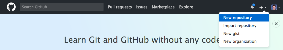
Let’s start by sharing the changes we’ve made to our current project
with the world. Log in to GitHub, then click on the icon in the top
right corner to create a new repository called
data-carpentry:
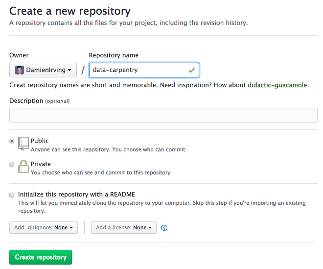
Name your repository “data-carpentry” and then click “Create Repository”:
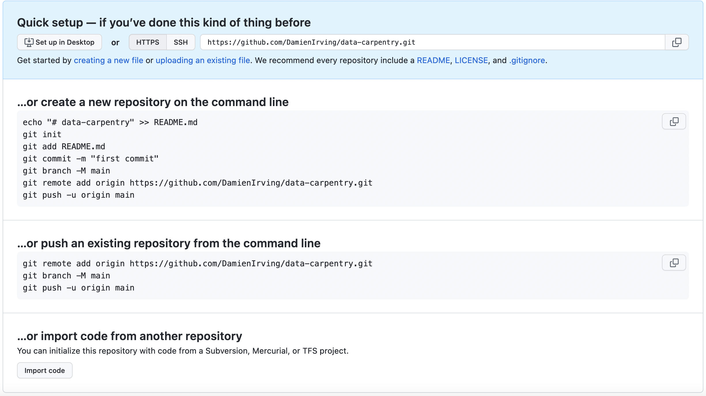
As soon as the repository is created, GitHub displays a page with a URL and some information on how to configure your local repository:
This effectively does the following on GitHub’s servers:
Our local repository still contains our earlier work on
plot_precipitation_climatology.py, but the remote
repository on GitHub doesn’t contain any files yet.
The next step is to connect the two repositories. We do this by making the GitHub repository a “remote” for the local repository. The home page of the repository on GitHub includes the string we need to identify it:
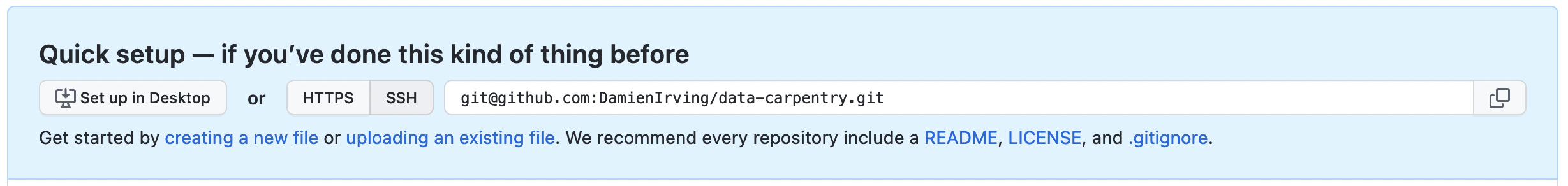
Click on the ‘SSH’ link to change the protocol from HTTPS to SSH if SSH isn’t already selected.
HTTPS vs. SSH
We use SSH here because, while it requires some additional configuration, it is a security protocol widely used by many applications. If you want to use HTTPS instead, you’ll need to create a Personal Access Token.
Copy that location from the browser, go into the local
data-carpentry repository, and run this command:
Make sure to use the location for your repository rather than
Damien’s: the only difference should be your username instead of
DamienIrving.
We can check that the command has worked by running
git remote -v:
OUTPUT
origin   git@github.com/DamienIrving/data-carpentry.git (push)
origin   git@github.com/DamienIrving/data-carpentry.git (fetch)
The name origin is a local nickname for your remote
repository. We could use something else if we wanted to, but
origin is by far the most common choice.
Connecting to GitHub with SSH
Before we can connect to our remote repository, we need to set up a way for our computer to authenticate with GitHub so it knows it’s us trying to connect to our remote repository.
We are going to set up the method that is commonly used by many different services to authenticate access on the command line. This method is called Secure Shell Protocol (SSH). SSH is a cryptographic network protocol that allows secure communication between computers using an otherwise insecure network.
SSH uses what is called a key pair. This is two keys that work together to validate access. One key is publicly known and called the public key, and the other key called the private key is kept private. Very descriptive names.
You can think of the public key as a padlock, and only you have the key (the private key) to open it. You use the public key where you want a secure method of communication, such as your GitHub account. You give this padlock, or public key, to GitHub and say “lock the communications to my account with this so that only computers that have my private key can unlock communications and send git commands as my GitHub account.”
What we will do now is the minimum required to set up the SSH keys and add the public key to a GitHub account.
Keeping your keys secure
You shouldn’t really forget about your SSH keys, since they keep your account secure. It’s good practice to audit your secure shell keys every so often. Especially if you are using multiple computers to access your account.
The first thing we are going to do is check if this has already been done on the computer we’re on. Because generally speaking, this setup only needs to happen once and then you can forget about it. We can run the list command to check what key pairs already exist on our computer.
(Your output is going to look a little different depending on whether or not SSH has ever been set up on the computer you are using.)
I have not set up SSH on my computer, so my output is
OUTPUT
ls: cannot access '/home/damien/.ssh': No such file or directoryIf SSH has been set up on the computer you’re using, the public and
private key pairs will be listed. The file names are either
id_ed25519/id_ed25519.pub or
id_rsa/id_rsa.pub depending on how the key
pairs were set up.
If they don’t exist on your computer, you can use this command to create them.
The -t option specifies which type of algorithm to use
and -C attaches a comment to the key (here, your
email).
If you are using a legacy system that doesn’t support the Ed25519
algorithm, use:$ ssh-keygen -t rsa -b 4096 -C "you@email.com"
OUTPUT
Generating public/private ed25519 key pair.
Enter file in which to save the key (/home/damien/.ssh/id_ed25519):
We want to use the default file, so just press Enter.
OUTPUT
Created directory '/home/damien/.ssh'.
Enter passphrase (empty for no passphrase):
Now, it is prompting us for a passphrase. If you’re using a laptop that other people sometimes have access to, you might want to create a passphrase. Be sure to use something memorable or save your passphrase somewhere, as there is no “reset my password” option.
OUTPUT
Enter same passphrase again:After entering the same passphrase a second time, we receive the confirmation.
OUTPUT
Your identification has been saved in /home/damien/.ssh/id_ed25519
Your public key has been saved in /home/damien/.ssh/id_ed25519.pub
The key fingerprint is:
SHA256:SMSPIStNyA00KPxuYu94KpZgRAYjgt9g4BA4kFy3g1o you@email.com
The key's randomart image is:
+--[ED25519 256]--+
|^B== o.          |
|%*=.*.+          |
|+=.E =.+         |
| .=.+.o..        |
|....  . S        |
|.+ o             |
|+ =              |
|.o.o             |
|oo+.             |
+----[SHA256]-----+
The “identification” is actually the private key. You should never share it. The public key is appropriately named. The “key fingerprint” is a shorter version of a public key.
Now that we have generated the SSH keys, we will find the SSH files when we check.
OUTPUT
drwxr-xr-x 1 Damien  staff  197121   0 Jul 16 14:48 ./
drwxr-xr-x 1 Damien  staff  197121   0 Jul 16 14:48 ../
-rw-r--r-- 1 Damien  staff  197121 419 Jul 16 14:48 id_ed25519
-rw-r--r-- 1 Damien  staff  197121 106 Jul 16 14:48 id_ed25519.pub
Now we have a SSH key pair and we can run this command to check if GitHub can read our authentication.
OUTPUT
The authenticity of host 'github.com (192.30.255.112)' can't be established.
RSA key fingerprint is SHA256:nThbg6kXUpJWGl7E1IGOCspRomTxdCARLviKw6E5SY8.
This key is not known by any other names
Are you sure you want to continue connecting (yes/no/[fingerprint])? y
Please type 'yes', 'no' or the fingerprint: yes
Warning: Permanently added 'github.com' (RSA) to the list of known hosts.
git@github.com: Permission denied (publickey).
Right, we forgot that we need to give GitHub our public key!
First, we need to copy the public key. Be sure to include the
.pub at the end, otherwise you’re looking at the private
key.
OUTPUT
ssh-ed25519 AAAAC3NzaC1lZDI1NTE5AAAAIDmRA3d51X0uu9wXek559gfn6UFNF69yZjChyBIU2qKI you@email.comNow, going to GitHub.com, click on your profile icon in the top right corner to get the drop-down menu. Click “Settings,” then on the settings page, click “SSH and GPG keys,” on the left side “Account settings” menu. Click the “New SSH key” button on the right side. Now, you can add a title (e.g. “work laptop” so you can remember where the original key pair files are located), paste your SSH key into the field, and click the “Add SSH key” to complete the setup.
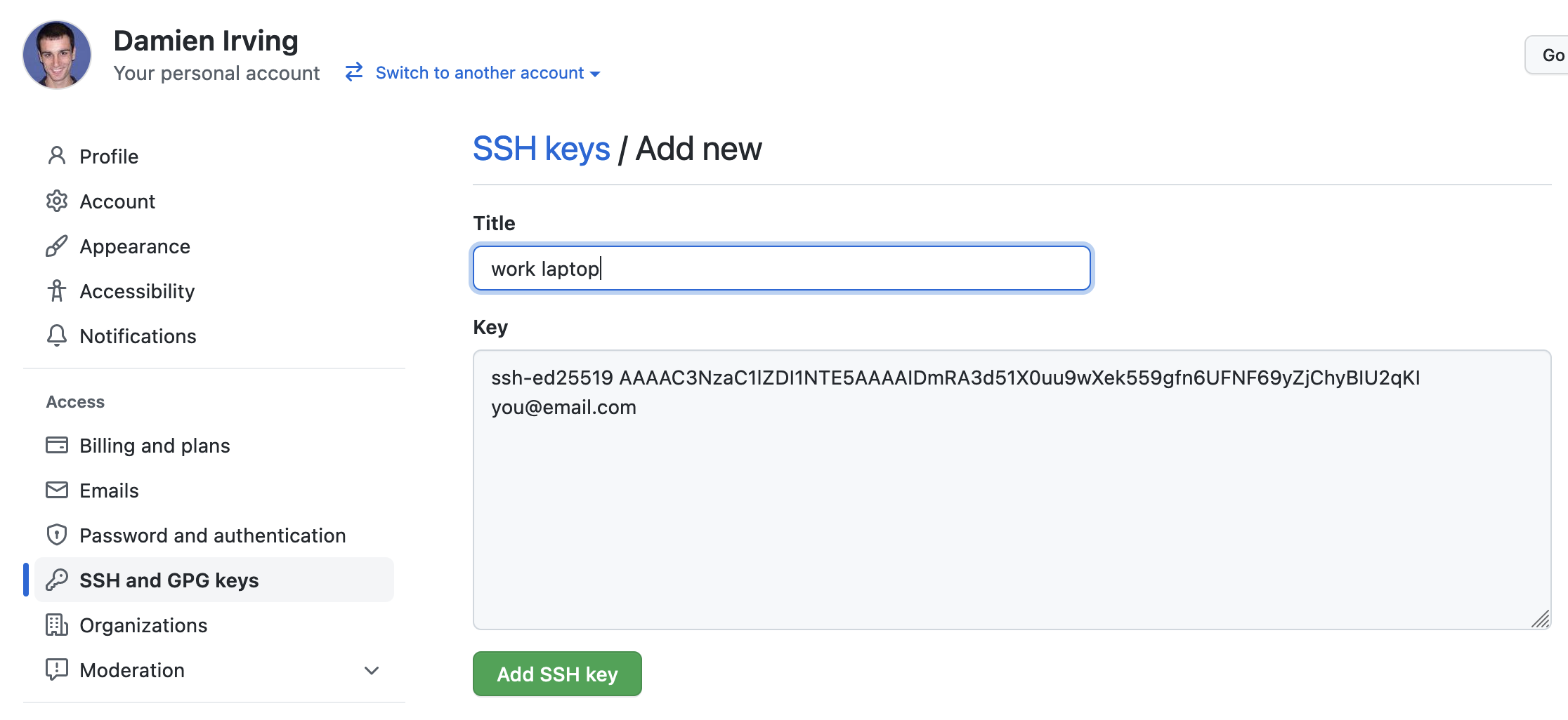
Now that we’ve set that up, let’s check our authentication again from the command line.
OUTPUT
Hi Damien! You've successfully authenticated, but GitHub does not provide shell access.Good! This output confirms that the SSH key works as intended. We are now ready to push our work to the remote repository.
OUTPUT
Counting objects: 9, done.
Delta compression using up to 4 threads.
Compressing objects: 100% (6/6), done.
Writing objects: 100% (9/9), 821 bytes, done.
Total 9 (delta 2), reused 0 (delta 0)
To github.com:DamienIrving/data-carpentry.git
 * [new branch]      master -> master
Branch master set up to track remote branch master from origin.
We can pull changes from the remote repository to the local one as well:
OUTPUT
From github.com:DamienIrving/data-carpentry.git
 * branch            master     -> FETCH_HEAD
Already up-to-date.
Pulling has no effect in this case because the two repositories are already synchronised. If someone else had pushed some changes to the repository on GitHub, though, this command would download them to our local repository.
Sharing code with yourself or others
If we logged onto a different computer (e.g. a supercomputing facility or our desktop computer at home) we could access a copy of our code by “cloning” it.
Since our repository is public, anyone (e.g. research collaborators) could clone the repository by getting the location from the corresponding page on GitHub:
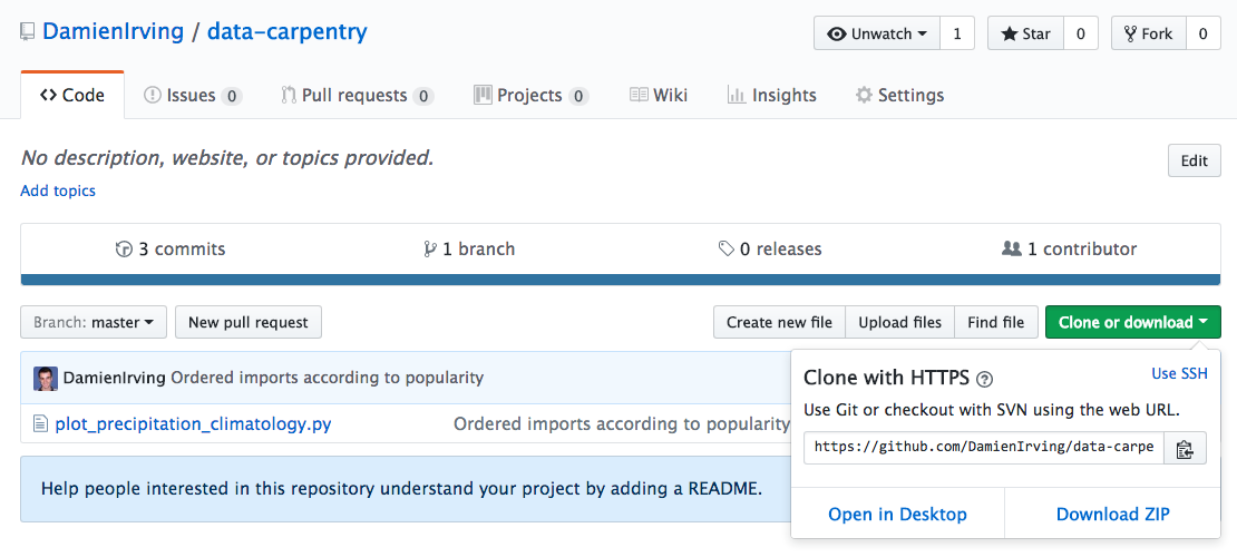
Working with others
Someone who clones your repository can’t push changes directly to it (unless you add them as a collaborator). They could, however, “fork” your repository and submit suggested changes via a “pull request”. Collaborators and pull requests are beyond the scope of this lesson, but you may come across them as you get more experienced with using git and GitHub.
Key Points
- A local Git repository can be connected to one or more remote repositories.
- You can use the SSH protocol to connect to remote repositories.
-
git pushcopies changes from a local repository to a remote repository. -
git pullcopies changes from a remote repository to a local repository.
Content from Vectorisation
Last updated on 2024-07-25 | Edit this page
Estimated time: 30 minutes
Overview
Questions
- How can I avoid looping over each element of large data arrays?
Objectives
- Use surface land fraction data to mask the land or ocean.
- Use the vectorised operations available in the
numpylibrary to avoid looping over array elements.
A useful addition to our
plot_precipitation_climatology.py script would be the
option to apply a land or ocean mask. To do this, we need to use the
land area fraction file.
PYTHON
import numpy as np
import xarray as xr


accesscm2_sftlf_file = "data/sftlf_fx_ACCESS-CM2_historical_r1i1p1f1_gn.nc"

ds = xr.open_dataset(accesscm2_sftlf_file)
sftlf = ds["sftlf"]
print(sftlf)
OUTPUT
<xarray.DataArray 'sftlf' (lat: 144, lon: 192)>
array([[100., 100., 100., ..., 100., 100., 100.],
       [100., 100., 100., ..., 100., 100., 100.],
       [100., 100., 100., ..., 100., 100., 100.],
       ...,
       [  0.,   0.,   0., ...,   0.,   0.,   0.],
       [  0.,   0.,   0., ...,   0.,   0.,   0.],
       [  0.,   0.,   0., ...,   0.,   0.,   0.]], dtype=float32)
Coordinates:
  * lat      (lat) float64 -89.38 -88.12 -86.88 -85.62 ... 86.88 88.12 89.38
  * lon      (lon) float64 0.9375 2.812 4.688 6.562 ... 353.4 355.3 357.2 359.1
Attributes:
    standard_name:   land_area_fraction
    long_name:       Percentage of the grid  cell occupied by land (including...
    comment:         Percentage of horizontal area occupied by land.
    units:           %
    original_units:  1
    history:         2019-11-09T02:47:20Z altered by CMOR: Converted units fr...
    cell_methods:    area: mean
    cell_measures:   area: areacella
The data in a sftlf file assigns each grid cell a percentage value between 0% (no land) to 100% (all land).
OUTPUT
100.0
0.0
To apply a mask to our plot, the value of all the data points we’d
like to mask needs to be set to np.nan. The most obvious
solution to applying a land mask, for example, might therefore be to
loop over each cell in our data array and decide whether it is a land
point (and thus needs to be set to np.nan).
(For this example, we are going to define land as any grid point that is more than 50% land.)
PYTHON
ds = xr.open_dataset("data/pr_Amon_ACCESS-CM2_historical_r1i1p1f1_gn_201001-201412.nc")
clim = ds['pr'].mean("time", keep_attrs=True)

nlats, nlons = clim.data.shape
for y in range(nlats):
    for x in range(nlons):
        if sftlf.data[y, x] > 50:
            clim.data[y, x] = np.nan
While this approach technically works, the problem is that (a) the code is hard to read, and (b) in contrast to low level languages like Fortran and C, high level languages like Python and Matlab are built for usability (i.e. they make it easy to write concise, readable code) as opposed to speed. This particular array is so small that the looping isn’t noticably slow, but in general looping over every data point in an array should be avoided.
Fortunately, there are lots of numpy functions (which are written in
C under the hood) that allow you to get around this problem by applying
a particular operation to an entire array at once (which is known as a
vectorised operation). The np.where function, for instance,
allows you to make a true/false decision at each data point in the array
and then perform a different action depending on the answer.
The developers of xarray have built-in the np.where
functionality, so creating a new DataArray with the land masked becomes
a one-line command:
OUTPUT
<xarray.DataArray 'pr' (lat: 144, lon: 192)>
array([[          nan,           nan,           nan, ...,           nan,
                  nan,           nan],
       [          nan,           nan,           nan, ...,           nan,
                  nan,           nan],
       [          nan,           nan,           nan, ...,           nan,
                  nan,           nan],
       ...,
       [7.5109556e-06, 7.4777777e-06, 7.4689174e-06, ..., 7.3359679e-06,
        7.3987890e-06, 7.3978440e-06],
       [7.1837171e-06, 7.1722038e-06, 7.1926393e-06, ..., 7.1552149e-06,
        7.1576678e-06, 7.1592167e-06],
       [7.0353467e-06, 7.0403985e-06, 7.0326828e-06, ..., 7.0392648e-06,
        7.0387587e-06, 7.0304386e-06]], dtype=float32)
Coordinates:
  * lon      (lon) float64 0.9375 2.812 4.688 6.562 ... 353.4 355.3 357.2 359.1
  * lat      (lat) float64 -89.38 -88.12 -86.88 -85.62 ... 86.88 88.12 89.38
Attributes:
    standard_name:  precipitation_flux
    long_name:      Precipitation
    units:          kg m-2 s-1
    comment:        includes both liquid and solid phases
    cell_methods:   area: time: mean
    cell_measures:  area: areacella
Mask option
Modify plot_precipitation_climatology.py so that the
user can choose to apply a mask via the following argparse
option:
PYTHON
parser.add_argument(
    "--mask",
    type=str,
    nargs=2,
    metavar=("SFTLF_FILE", "REALM"),
    default=None,
    help="""Provide sftlf file and realm to mask ('land' or 'ocean')""",
)
This should involve defining a new function called
apply_mask(), in order to keep main() short
and readable.
Test to see if your mask worked by plotting the ACCESS-CM2 climatology for JJA:
BASH
$ python plot_precipitation_climatology.py data/pr_Amon_ACCESS-CM2_historical_r1i1p1f1_gn_201001-201412.nc JJA pr_Amon_ACCESS-CM2_historical_r1i1p1f1_gn_201001-201412-JJA-clim_land-mask.png --mask data/sftlf_fx_ACCESS-CM2_historical_r1i1p1f1_gn.nc ocean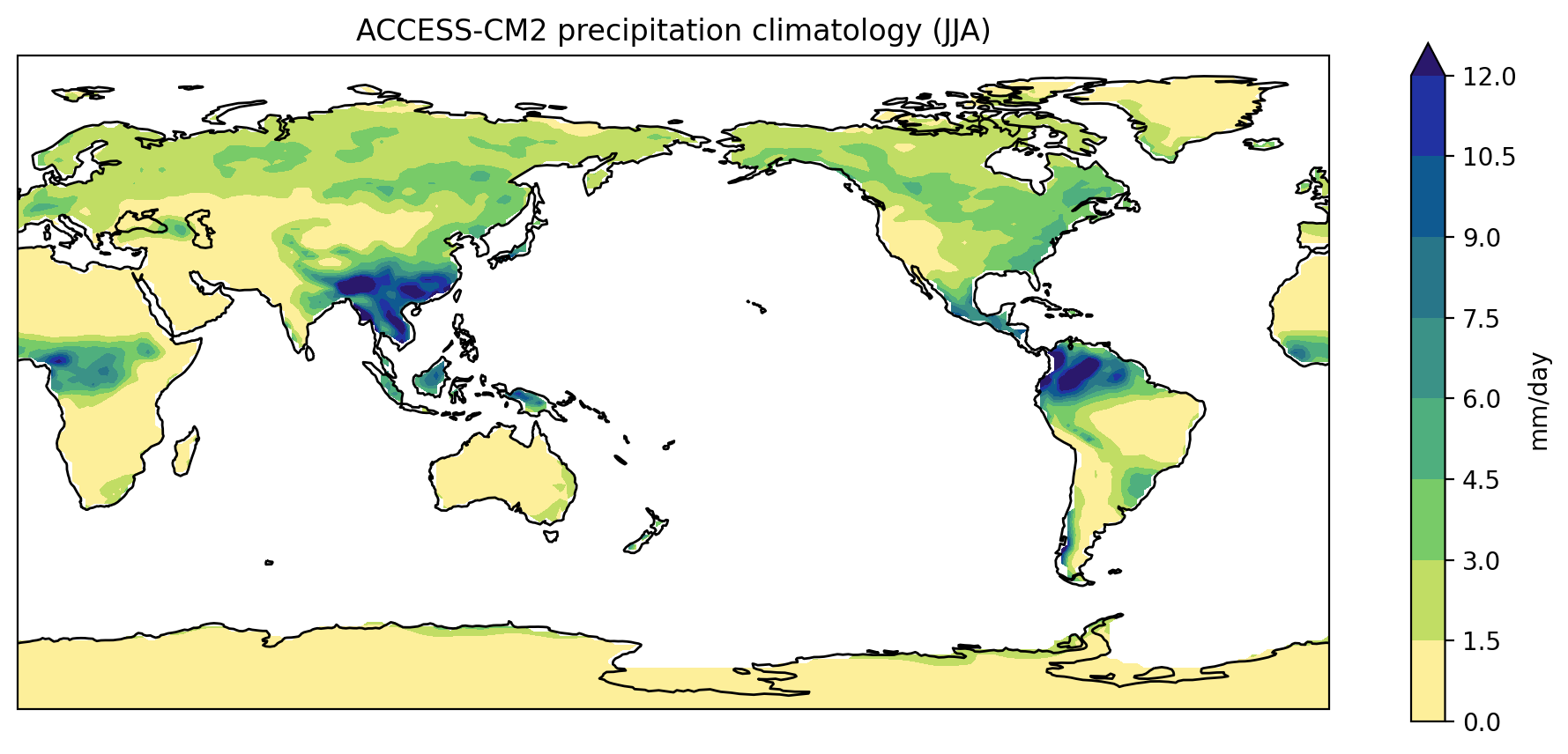
Commit the changes to git and then push to GitHub.
Make the following additions to
plot_precipitation_climatology.py (code omitted from this
abbreviated version of the script is denoted ...):
PYTHON
def apply_mask(da, sftlf_file, realm):
    """Mask ocean or land using a sftlf (land surface fraction) file.

    Args:
     da (xarray.DataArray): Data to mask
     sftlf_file (str): Land surface fraction file
     realm (str): Realm to mask

    """

    ds = xr.open_dataset(sftlf_file)

    if realm == 'land':
        masked_da = da.where(ds['sftlf'].data < 50)
    else:
        masked_da = da.where(ds['sftlf'].data > 50)

    return masked_da

...

def main(inargs):
    """Run the program."""

    ds = xr.open_dataset(inargs.pr_file)

    clim = ds["pr"].groupby("time.season").mean("time", keep_attrs=True)
    clim = convert_pr_units(clim)

    if inargs.mask:
        sftlf_file, realm = inargs.mask
        clim = apply_mask(clim, sftlf_file, realm)

    ...

if __name__ == "__main__":

    description = "Plot the precipitation climatology for a given season."
    parser = argparse.ArgumentParser(description=description)

    ...

    parser.add_argument(
        "--mask",
        type=str,
        nargs=2,
        metavar=("SFTLF_FILE", "REALM"),
        default=None,
        help="""Provide sftlf file and realm to mask ('land' or 'ocean')""",
    )

    args = parser.parse_args()
    main(args)
plot_precipitation_climatology.py
At the conclusion of this lesson your
plot_precipitation_climatology.py script should look
something like the following:
PYTHON
import argparse

import xarray as xr
import cartopy.crs as ccrs
import matplotlib.pyplot as plt
import numpy as np
import cmocean


def convert_pr_units(da):
    """Convert kg m-2 s-1 to mm day-1.

    Args:
      da (xarray.DataArray): Precipitation data

    """

    da.data = da.data * 86400
    da.attrs["units"] = "mm/day"

    return da


def apply_mask(da, sftlf_file, realm):
    """Mask ocean or land using a sftlf (land surface fraction) file.

    Args:
      da (xarray.DataArray): Data to mask
      sftlf_file (str): Land surface fraction file
      realm (str): Realm to mask

    """

    ds = xr.open_dataset(sftlf_file)

    if realm == 'land':
        masked_da = da.where(ds['sftlf'].data < 50)
    else:
        masked_da = da.where(ds['sftlf'].data > 50)

    return masked_da


def create_plot(clim, model, season, gridlines=False, levels=None):
    """Plot the precipitation climatology.

    Args:
      clim (xarray.DataArray): Precipitation climatology data
      model (str): Name of the climate model
      season (str): Season

    Kwargs:
      gridlines (bool): Select whether to plot gridlines
      levels (list): Tick marks on the colorbar

    """

    if not levels:
        levels = np.arange(0, 13.5, 1.5)

    fig = plt.figure(figsize=[12,5])
    ax = fig.add_subplot(111, projection=ccrs.PlateCarree(central_longitude=180))
    clim.sel(season=season).plot.contourf(
        ax=ax,
        levels=levels,
        extend="max",
        transform=ccrs.PlateCarree(),
        cbar_kwargs={"label": clim.units},
        cmap=cmocean.cm.haline_r
    )
    ax.coastlines()
    if gridlines:
        plt.gca().gridlines()

    title = f"{model} precipitation climatology ({season})"
    plt.title(title)


def main(inargs):
    """Run the program."""

    ds = xr.open_dataset(inargs.pr_file)

    clim = ds["pr"].groupby("time.season").mean("time", keep_attrs=True)
    clim = convert_pr_units(clim)

    if inargs.mask:
        sftlf_file, realm = inargs.mask
        clim = apply_mask(clim, sftlf_file, realm)

    create_plot(
        clim,
        ds.attrs["source_id"],
        inargs.season,
        gridlines=inargs.gridlines,
        levels=inargs.cbar_levels
    )
    plt.savefig(
        inargs.output_file,
        dpi=200,
        bbox_inches="tight",
        facecolor="white",
    )


if __name__ == "__main__":
    description = "Plot the precipitation climatology for a given season."
    parser = argparse.ArgumentParser(description=description)

    parser.add_argument("pr_file", type=str, help="Precipitation data file")
    parser.add_argument("season", type=str, help="Season to plot")
    parser.add_argument("output_file", type=str, help="Output file name")

    parser.add_argument(
        "--gridlines",
        action="store_true",
        default=False,
        help="Include gridlines on the plot",
    )
    parser.add_argument(
        "--cbar_levels",
        type=float,
        nargs="*",
        default=None,
        help="list of levels / tick marks to appear on the colorbar",
    )
    parser.add_argument(
        "--mask",
        type=str,
        nargs=2,
        metavar=("SFTLF_FILE", "REALM"),
        default=None,
        help="""Provide sftlf file and realm to mask ('land' or 'ocean')""",
    )

    args = parser.parse_args()
    main(args)
Key Points
- For large arrays, looping over each element can be slow in high-level languages like Python.
- Vectorised operations can be used to avoid looping over array elements.
Content from Defensive programming
Last updated on 2024-07-25 | Edit this page
Estimated time: 30 minutes
Overview
Questions
- How can I make my programs more reliable?
Objectives
- Signal errors by raising exceptions.
- Use try-except blocks to catch and handle exceptions.
- Explain what an assertion is.
- Add assertions that check the program’s state is correct.
- Use a logging framework to report on program activity.
- Identify sources of more advanced lessons on code testing.
Scientist’s nightmare
If you needed any motivation to learn and employ the principles of defensive programming, look no further than this article. It documents the experience of a researcher who had to retract five published papers - three of which were in Science - because his code had inadvertently switched the rows and columns of a data table.
Now that we’ve written
plot_precipitation_climatology.py, how can we be sure that
it’s producing reliable results?
The first step toward getting the right answers from our programs is to assume that mistakes will happen and to guard against them. This is called defensive programming, and there are a number of tools and approaches at our disposal for doing this. Broadly speaking, we can raise and handle errors to check and respond to program inputs, use assertions to make sure nothing crazy or unexpected has happened, write unit tests to make sure each component of our program produces expected outputs, and use a logging framework to report on program activity. In this lesson, we’ll look at how error handling, assertions and logging can make the unit conversion in our program more reliable, and we’ll provide links to further information on unit .
Types of errors
There are essentially two kinds of errors that can arise in Python: syntax errors and exceptions. You’re probably familiar with the former:
ERROR
    if rainfall > 10
                    ^
SyntaxError: expected ':'
Once a statement or expression is syntactically correct, it may cause an error when an attempt is made to execute it. Errors detected during execution are called exceptions (i.e. an exception from normal behaviour) and there are lots of different types of exceptions:
ERROR
ZeroDivisionError: division by zeroERROR
NameError: name 'spam' is not definedERROR
TypeError: can only concatenate str (not "int") to strRaising errors
With respect to defensive programming, it can sometimes be useful to
raise your own exceptions (using the raise keyword).
PYTHON
infile = "temperature_data.txt"
file_format = infile.split(".")[-1]
if file_format != "nc":
    raise ValueError(f"{infile} does not have the netCDF file extension .nc")
ERROR
ValueError                                Traceback (most recent call last)
/var/folders/6v/vrpsky6j509dff7250jyg8240000gp/T/ipykernel_12425/3612736507.py in <module>
      2 file_format = infile.split(".")[-1]
      3 if file_format != "nc":
----> 4     raise ValueError(f"{infile} does not have the netCDF file extension .nc")

ValueError: temperature_data.txt does not have the netCDF file extension .nc
In this case we’ve chosen to raise a ValueError, but we
could pick any of the builtin
exception types (including just a generic Exception) or
define our own custom
exception class.
In the context of our plot_precipitation_climatology.py
script, we currently multiply our data by 86400 regardless of what the
input units are. It would be better if we modified the main
function so that the program multiplied by 86400 if the input units are
kg m-2 s-1, performed no unit conversion if the input units are mm/day,
or halted with an informative error message if the input data have some
other units.
Handling errors
As we’ve seen in the examples above, if exceptions aren’t dealt with
the program crashes. The error message upon crashing is sometimes be
easy to understand (particularly if you wrote the raise
statement yourself) but can often be cryptic.
If we’d rather the program didn’t crash when a particular exception occurs, we can use a try-except block to catch and handle the exception. The syntax of the try-except block is:
The code in the except block is only executed if an exception
occurred in the try block. The except block is required with a try
block, even if it contains only the pass statement
(i.e. ignore the exception and carry on). For example, let’s say there’s
a calculation in our program where we need to divide by the number of
available weather stations. If there were no weather stations available,
by default the program would crash.
ERROR
ZeroDivisionError                         Traceback (most recent call last)
/var/folders/6v/vrpsky6j509dff7250jyg8240000gp/T/ipykernel_12425/3927438267.py in <module>
      2 n_stations = 0
      3
----> 4 scaled_quantity = quantity / n_stations
      5 print(scaled_quantity)

ZeroDivisionError: division by zero
If we’d prefer the program simply continue with a
scaled_quantity value of NaN, we could catch and handle the
ZeroDivisionError.
PYTHON
import numpy as np


quantity = 500
n_stations = 0

try:
    scaled_quantity = quantity / n_stations
except ZeroDivisionError:
    scaled_quantity = np.nan

print(scaled_quantity)
OUTPUT
nanIn the context of our plot_precipitation_climatology.py
script, the variable attributes from the input netCDF file are stored in
a dictionary that we access via clim.attrs. The dictionary
keys are the names of the variable attributes
(e.g. standard_name, long_name,
units) and the dictionary values are the values
corresponding to those keys (e.g. precipitation_flux,
Precipitation, kg m-2 s-1). If the input data
file didn’t have a units attribute associated with the precipitation
variable, our program would currently fail with a KeyError
(which Python raises when you ask for a key that isn’t in a
dictionary).
PYTHON
example_dict = {
    "standard_name": "precipitation_flux",
    "long_name": "Precipitation",
}
units = example_dict["units"]
ERROR
KeyError                                  Traceback (most recent call last)
/var/folders/6v/vrpsky6j509dff7250jyg8240000gp/T/ipykernel_12425/2679443625.py in <module>
      1 example_dict = {
      2     "standard_name": "precipitation_flux",
      3     "long_name": "Precipitation",
      4 }
----> 5 units = example_dict["units"]

KeyError: 'units'
It’s fine that our program would crash in this situation (we can’t
continue if we don’t know the units of the input data), but the error
message doesn’t explicitly tell the user that the input file requires a
units attribute. To make this crystal clear, we could use a try-except
block in the main function to catch the
KeyError and re-define a better error message.
Assertions
Unexpected behaviour in a program can sometimes propagate a long way before triggering an exception or producing a perplexing result. For instance, if a calculation produces a non-physical value for precipitation (e.g. a negative value) that value could be used in various downstream calculations of drought and fire risk (combined with values for temperature, wind, humidity, etc). The final plot of the forest fire danger index might look wrong (or not, which would be even worse) to the scientist who wrote and executed the code, but it wouldn’t be immediately obvious that the precipitation calculation was the source of the problem.
In order to avoid propagation, it’s best to nip unexpected behaviour
in the bud right when it occurs. One way to do this is to add assertions
to your code. An assertion is simply a statement that something must be
true at a certain point in a program. When Python sees one, it evaluates
the assertion’s condition. If it’s true, Python does nothing, but if
it’s false, Python halts the program immediately and raises an
AssertionError with a custom error message.
To demonstrate an assertion in action, consider this piece of code that halts if any precipitation data is negative:
PYTHON
import numpy as np
pr_data = np.array([1.5, 2.3, 0.7, -0.2, 4.4])
assert pr_data.min() >= 0.0, "There is at least one negative precipitation value"ERROR
---------------------------------------------------------------------------
AssertionError Traceback (most recent call last)
<ipython-input-19-33d87ea29ae4> in <module>()
----> 1 assert pr_data.min() >= 0.0, "There is at least one negative precipitation value"
AssertionError: There is at least one negative precipitation valueWith respect to our command line program, one thing to check would be
that the climatological precipitation values lie within a sensible range
after the unit conversion. The world
record highest daily rainfall total is 1825mm (at Reunion Island in
1966), so climatological values across the globe should be more than 0
but less than 2000 mm/day. We could add the following assertions to our
convert_pr_units function to catch unexpected precipitation
values.
PYTHON
assert darray.data.min() >= 0.0, "There is at least one negative precipitation value"
assert darray.data.max() < 2000, "There is a precipitation value/s > 2000 mm/day"Assertions are also used in unit testing (each test culminates in an assertion), but that topic is beyond the scope of this lesson.
Testing and continuous integration
An assertion checks that something is true at a particular point in
the program. For programs that are more complex (or research critical)
than plot_precipitation_climatology.py, it’s a good idea to
take the next step and check the overall behavior of entire pieces (or
units) of code. Related concepts like unit testing and continuous
integration are beyond the scope of this lesson, but Research
Software Engineering With Python has a chapter on testing
that is well worth a read.
Logging
So far we’ve considered how to make our programs halt or handle the situation when things go wrong. Another option in our defensive programming toolkit is to have our programs report their own activity.
For example, let’s say we’re working with relative humidity data. We wouldn’t typically expect to encounter any values over 100%, but it is physically possible. Rather than halt the program if a value over 100% occurs, we might therefore want our program to simply report the maximum relative humidity. We can then decide whether to trust the output or not (e.g. a value of 100.1% might be ok but not 150%).
To do this reporting, our first instinct might be to add a
print statement to the program.
PYTHON
rh_data = np.array([1.5, 20.4, 100.1, 76.3, 54.4])
rh_max = rh_data.max()
print(f"The maximum relative humidity was {rh_max}%")OUTPUT
The maximum relative humidity was 100.1%The problem with this approach is that information printed to the
screen is lost once we close our command line session. Constantly
adding, removing or commenting out print statements is also
tedious and error-prone.
A better approach is to use a logging framework, such as Python’s
logging library. This lets us leave debugging statements in
our code and turn them on or off at will. Let’s start by replacing our
print statement with a logging command.
PYTHON
import logging
rh_data = np.array([1.5, 20.4, 100.1, 76.3, 54.4])
rh_max = rh_data.max()
logging.debug(f"The maximum relative humidity was {rh_max}%")Whoops! There’s no output because by default the logging library only reports information at the “warning” level and above. In order of increasing severity, the available levels are:
-
debug: very detailed information used for localizing errors. -
info: confirmation that things are working as expected. -
warning: something unexpected happened, but the program will keep going. -
error: something has gone badly wrong, but the program hasn’t hurt anything. -
critical: potential loss of data, security breach, etc.
If we want to see the output from less severe levels (i.e. turn our debugging statements on), we’d need to change the minimum level in the logging configuration. We can also provide the name of a file to write the logging information to, so that it isn’t lost when we finish our command line session.
PYTHON
# for loop only required in notebooks
for handler in logging.root.handlers[:]:
logging.root.removeHandler(handler)
logging.basicConfig(level=logging.DEBUG, filename="log.txt"))
rh_data = np.array([1.5, 20.4, 100.1, 76.3, 54.4])
rh_max = rh_data.max()
logging.debug(f"The maximum relative humidity was {rh_max}%")(The for loop is needed to turn off the background logging the notebook does itself. It’s not needed in a Python script.)
Notice that we’ve used capital logging.DEBUG (which is
an integer value) to set the logging level, as opposed to the
logging.debug function that is used for logging a
message.
By setting the logging level to “DEBUG”, our output “log.txt” file will now capture all logging information with a flag of ‘debug’ or higher - that is, all logging outputs will be written to our log file.
OUTPUT
DEBUG:root:The maximum relative humidity was 100.1%In the context of the plot_precipitation_climatology.py
script, it would be nice to know whether or not unit conversion was
performed. To do this we just need a few small changes to the script. We
need to import the logging library at the top of the script,
and set the logging configuration and add a logging.info
command in the main function.
PYTHON
def main(inargs):
"""Run the program."""
logging.basicConfig(level=logging.DEBUG, filename="log.txt")
...
if input_units == 'kg m-2 s-1':
clim = convert_pr_units(clim)
logging.info("Units converted from kg m-2 s-1 to mm/day")
elif input_units == "mm/day":
pass
else:
raise ValueError("""Input units are not 'kg m-2 s-1' or 'mm/day'""")
...Update your script
Update your working copy of
plot_precipitation_climatology.py with the changes from
this lesson.
This will mean your main function will now read as
follows,
PYTHON
def main(inargs):
"""Run the program."""
logging.basicConfig(level=logging.DEBUG, filename="log.txt")
ds = xr.open_dataset(inargs.pr_file)
clim = ds["pr"].groupby("time.season").mean("time", keep_attrs=True)
try:
input_units = clim.attrs["units"]
except KeyError:
raise KeyError(f"Precipitation variable in {inargs.pr_file} must have a units attribute")
if input_units == "kg m-2 s-1":
clim = convert_pr_units(clim)
logging.info("Units converted from kg m-2 s-1 to mm/day")
elif input_units == "mm/day":
pass
else:
raise ValueError("""Input units are not 'kg m-2 s-1' or 'mm/day'""")
if inargs.mask:
sftlf_file, realm = inargs.mask
clim = apply_mask(clim, sftlf_file, realm)
create_plot(
clim,
dset.attrs["source_id"],
inargs.season,
gridlines=inargs.gridlines,
levels=inargs.cbar_levels
)
plt.savefig(
inargs.output_file,
dpi=200,
bbox_inches="tight",
facecolor="white",
)and your convert_pr_units as:
PYTHON
def convert_pr_units(da):
"""Convert kg m-2 s-1 to mm day-1.
Args:
da (xarray.DataArray): Precipitation data
"""
da.data = da.data * 86400
da.attrs["units"] = "mm/day"
assert da.data.min() >= 0.0, "There is at least one negative precipitation value"
assert da.data.max() < 2000, "There is a precipitation value/s > 2000 mm/day"
return daVerbose reporting
Add two new command line options to
plot_precipitation_climatology.py.
The first should change the logging level so reporting from the program is more verbose.
PYTHON
parser.add_argument(
"-v",
"--verbose",
action="store_true",
default=False,
help="Change the minimum logging reporting level from WARNING (default) to INFO",
)The second should allow the user to specify the name of the log file. (If they don’t specify a name then the logging information is printed to the screen.)
Error handling for land/ocean masks
In the previous lesson we added an apply_mask function
to our script. Update the following if statement in that function so
that it raises a ValueError if the realm is not
ocean or land.
plot_precipitation_climatology.py
At the conclusion of this lesson your
plot_precipitation_climatology.py script should look
something like the following:
PYTHON
import logging
import argparse
import xarray as xr
import cartopy.crs as ccrs
import matplotlib.pyplot as plt
import numpy as np
import cmocean
def convert_pr_units(da):
"""Convert kg m-2 s-1 to mm day-1.
Args:
da (xarray.DataArray): Precipitation data
"""
da.data = da.data * 86400
da.attrs["units"] = "mm/day"
assert da.data.min() >= 0.0, "There is at least one negative precipitation value"
assert da.data.max() < 2000, "There is a precipitation value/s > 2000 mm/day"
return da
def apply_mask(da, sftlf_file, realm):
"""Mask ocean or land using a sftlf (land surface fraction) file.
Args:
da (xarray.DataArray): Data to mask
sftlf_file (str): Land surface fraction file
realm (str): Realm to mask
"""
ds = xr.open_dataset(sftlf_file)
if realm.lower() == "land":
masked_da = da.where(ds["sftlf"].data < 50)
elif realm.lower() == 'ocean':
masked_da = da.where(ds["sftlf"].data > 50)
else:
raise ValueError("""Mask realm is not 'ocean' or 'land'""")
return masked_da
def create_plot(clim, model, season, gridlines=False, levels=None):
"""Plot the precipitation climatology.
Args:
clim (xarray.DataArray): Precipitation climatology data
model (str): Name of the climate model
season (str): Season
Kwargs:
gridlines (bool): Select whether to plot gridlines
levels (list): Tick marks on the colorbar
"""
if not levels:
levels = np.arange(0, 13.5, 1.5)
fig = plt.figure(figsize=[12,5])
ax = fig.add_subplot(111, projection=ccrs.PlateCarree(central_longitude=180))
clim.sel(season=season).plot.contourf(
ax=ax,
levels=levels,
extend='max',
transform=ccrs.PlateCarree(),
cbar_kwargs={"label": clim.units},
cmap=cmocean.cm.haline_r,
)
ax.coastlines()
if gridlines:
plt.gca().gridlines()
title = f"{model} precipitation climatology ({season})"
plt.title(title)
def main(inargs):
"""Run the program."""
log_lev = logging.DEBUG if inargs.verbose else logging.WARNING
logging.basicConfig(level=log_lev, filename=inargs.logfile)
ds = xr.open_dataset(inargs.pr_file)
clim = ds['pr'].groupby("time.season").mean("time", keep_attrs=True)
try:
    input_units = clim.attrs["units"]
except KeyError:
    raise KeyError(f"Precipitation variable in {inargs.pr_file} does not have a units attribute")
if input_units == "kg m-2 s-1":
clim = convert_pr_units(clim)
logging.info("Units converted from kg m-2 s-1 to mm/day")
elif input_units == "mm/day":
pass
else:
raise ValueError("""Input units are not 'kg m-2 s-1' or 'mm/day'""")
if inargs.mask:
sftlf_file, realm = inargs.mask
clim = apply_mask(clim, sftlf_file, realm)
create_plot(
clim,
ds.attrs["source_id"],
inargs.season,
gridlines=inargs.gridlines,
levels=inargs.cbar_levels
)
plt.savefig(
inargs.output_file,
dpi=200,
bbox_inches="tight",
facecolor="white",
)
if __name__ == '__main__':
description='Plot the precipitation climatology for a given season.'
parser = argparse.ArgumentParser(description=description)
parser.add_argument("pr_file", type=str, help="Precipitation data file")
parser.add_argument("season", type=str, help="Season to plot")
parser.add_argument("output_file", type=str, help="Output file name")
parser.add_argument(
"--gridlines",
action="store_true",
default=False,
help="Include gridlines on the plot",
)
parser.add_argument(
"--cbar_levels",
type=float,
nargs="*",
default=None,
help="list of levels / tick marks to appear on the colorbar",
)
parser.add_argument(
"--mask",
type=str,
nargs=2,
metavar=("SFTLF_FILE", "REALM"),
default=None,
help="""Provide sftlf file and realm to mask ('land' or 'ocean')""",
)
parser.add_argument(
"-v",
"--verbose",
action="store_true",
default=False,
help="Change the minimum logging reporting level from WARNING (default) to DEBUG",
)
parser.add_argument(
"--logfile",
type=str,
default=None,
help="Name of log file (by default logging information is printed to the screen)",
)
args = parser.parse_args()
main(args)Key Points
- Program defensively, i.e., assume that errors are going to arise, and write code to detect them when they do.
- You can raise exceptions in your own code.
- Put try-except blocks in programs to catch and handle exceptions.
- Put assertions in programs to check their state as they run.
- Use a logging framework instead of
printstatements to report program activity. - The are more advanced lessons you can read to learn about code testing.
Content from Data provenance
Last updated on 2024-07-25 | Edit this page
Estimated time: 30 minutes
Overview
Questions
- How can keep track of my data processing steps?
Objectives
- Automate the process of recording the history of what was entered at the command line to produce a given data file or image.
We’ve now successfully created a command line program -
plot_precipitation_climatology.py - that calculates and
plots the precipitation climatology for a given season. The last step is
to capture the provenance of that plot. In other words, we need a log of
all the data processing steps that were taken from the intial download
of the data file to the end result (i.e. the PNG image).
The simplest way to do this is to follow the lead of the NCO and CDO command line tools, which insert a record of what was executed at the command line into the history attribute of the output netCDF file. If fact, they were both used in the pre-processing of the data files used in these lessons:
PYTHON
import xarray as xr
accessesm15_pr_file = "data/pr_Amon_ACCESS-ESM1-5_historical_r1i1p1f1_gn_201001-201412.nc"
ds = xr.open_dataset(accessesm15_pr_file)
print(ds.attrs['history'])OUTPUT
Tue Jan 12 14:50:35 2021: ncatted -O -a history,pr,d,, pr_Amon_ACCESS-ESM1-5_historical_r1i1p1f1_gn_201001-201412.nc
Tue Jan 12 14:48:10 2021: cdo seldate,2010-01-01,2014-12-31 /g/data/fs38/publications/CMIP6/CMIP/CSIRO/ACCESS-ESM1-5/historical/r1i1p1f1/Amon/pr/gn/latest/pr_Amon_ACCESS-ESM1-5_historical_r1i1p1f1_gn_185001-201412.nc pr_Amon_ACCESS-ESM1-5_historical_r1i1p1f1_gn_201001-201412.nc
2019-11-15T04:32:57Z ; CMOR rewrote data to be consistent with CMIP6, CF-1.7 CMIP-6.2 and CF standards.Fortunately, there is a Python package called cmdline-provenance that creates NCO/CDO-style records of what was executed at the command line. We can use it to add to the command log, before inserting the updated log into the metadata associated with our output image file.
To start, let’s import the cmdline_provenance library
with the other imports at the top of our
plot_precipitation_climatology.py script,
and then make the following updates to the original line of code responsible for saving the image to file:
PYTHON
new_log = cmdprov.new_log(infile_logs={inargs.pr_file: dset.attrs["history"]})
plt.savefig(
inargs.output_file,
metadata={"History": new_log},
dpi=200,
bbox_inches="tight",
facecolor="white",
)When we execute plot_precipitation_climatology.py,
cmdprov.new_log will create a record of what was entered at
the command line. The name of the input precipitation file and its
history attribute have been provided using the infile_logs
argument, so that cmdprov.new_log can append the history of
that file to the new command log. The metadata argument for
plt.savefig has then been used to save the new command log
to the image metadata.
To see this in action, we can run the program,
BASH
$ python plot_precipitation_climatology.py data/pr_Amon_ACCESS-ESM1-5_historical_r1i1p1f1_gn_201001-201412.nc SON pr_Amon_ACCESS-ESM1-5_historical_r1i1p1f1_gn_201001-201412-SON-clim.pngand then view the metadata of the new PNG image file. There are a
number of different programs available to do this, but they can often be
tricky to install. Fortunately, conda is used to install
programs written in many different languages, not just Python. There are
installation
recipes for a command line program called exiftool on anaconda.org,
so let’s go ahead and install that:
Once installed, we can use it to view the metadata associated with our image file:
OUTPUT
ExifTool Version Number : 12.17
File Name : pr_Amon_ACCESS-ESM1-5_historical_r1i1p1f1_gn_201001-201412-SON-clim.png
Directory : .
File Size : 315 KiB
File Modification Date/Time : 2021:02:08 10:16:56+11:00
File Access Date/Time : 2021:02:08 10:16:58+11:00
File Inode Change Date/Time : 2021:02:08 10:16:56+11:00
File Permissions : rw-r--r--
File Type : PNG
File Type Extension : png
MIME Type : image/png
Image Width : 2400
Image Height : 1000
Bit Depth : 8
Color Type : RGB with Alpha
Compression : Deflate/Inflate
Filter : Adaptive
Interlace : Noninterlaced
Software : Matplotlib version3.3.3, https://matplotlib.org/
History : Mon Feb 08 09:45:17 2021: /Users/damien/opt/anaconda3/envs/pyaos-lesson/bin/python code/plot_precipitation_climatology.py data/pr_Amon_ACCESS-ESM1-5_historical_r1i1p1f1_gn_201001-201412.nc SON pr_Amon_ACCESS-ESM1-5_historical_r1i1p1f1_gn_201001-201412-SON-clim.png.Tue Jan 12 14:50:35 2021: ncatted -O -a history,pr,d,, pr_Amon_ACCESS-ESM1-5_historical_r1i1p1f1_gn_201001-201412.nc.Tue Jan 12 14:48:10 2021: cdo seldate,2010-01-01,2014-12-31 /g/data/fs38/publications/CMIP6/CMIP/CSIRO/ACCESS-ESM1-5/historical/r1i1p1f1/Amon/pr/gn/latest/pr_Amon_ACCESS-ESM1-5_historical_r1i1p1f1_gn_185001-201412.nc pr_Amon_ACCESS-ESM1-5_historical_r1i1p1f1_gn_201001-201412.nc.2019-11-15T04:32:57Z ; CMOR rewrote data to be consistent with CMIP6, CF-1.7 CMIP-6.2 and CF standards. .
Pixels Per Unit X : 7874
Pixels Per Unit Y : 7874
Pixel Units : meters
Image Size : 2400x1000
Megapixels : 2.4Now that we’ve successfully added a command log to our PNG image, we might want to think about how our script should handle other image formats (e.g. PDF, EPS)? For PNG files you can pick whatever metadata keys you like (hence we picked “History”), but other formats only allow specific keys. For now we can add raise an error so that the program halts if someone tries to generate a format that isn’t PNG, and in the exercises we’ll add more valid formats to the script.
PYTHON
image_format = inargs.output_file.split(".")[-1])
if image_format != "png":
raise ValueError("Output file must have the PNG image file extension .png")Putting this altogether, here’s what the main function
in plot_precipitation_climatology.py looks like:
PYTHON
def main(inargs):
"""Run the program."""
log_lev = logging.DEBUG if inargs.verbose else logging.WARNING
logging.basicConfig(level=log_lev, filename=inargs.logfile)
ds = xr.open_dataset(inargs.pr_file)
clim = ds["pr"].groupby("time.season").mean("time", keep_attrs=True)
try:
input_units = clim.attrs["units"]
except KeyError:
raise KeyError(f"Precipitation variable in {inargs.pr_file} does not have a units attribute")
if input_units == "kg m-2 s-1":
clim = convert_pr_units(clim)
logging.info("Units converted from kg m-2 s-1 to mm/day")
elif input_units == "mm/day":
pass
else:
raise ValueError("""Input units are not 'kg m-2 s-1' or 'mm/day'""")
if inargs.mask:
sftlf_file, realm = inargs.mask
clim = apply_mask(clim, sftlf_file, realm)
create_plot(
clim,
ds.attrs["source_id"],
inargs.season,
gridlines=inargs.gridlines,
levels=inargs.cbar_levels,
)
image_format = inargs.output_file.split(".")[-1]
if image_format != "png":
raise ValueError("Output file must have the PNG image file extension .png")
new_log = cmdprov.new_log(infile_logs={inargs.pr_file: ds.attrs["history"]})
plt.savefig(
inargs.output_file,
metadata={"History": new_log},
dpi=200,
bbox_inches="tight",
facecolor="white",
)Handling different image formats
The plt.savefig
documentation provides information on the metadata keys accepted by
PNG, PDF, EPS and PS image formats.
Using that information as a guide, add a new function called
get_log_and_key to the
plot_precipitation_climatology.py script. It should take
the precipitation file name, history attribute, and plot type as
arguments and return the updated command log and the appropriate
metadata key for PNG, PDF, EPS or PS image formats.
When you’re done, the final lines of the main function
should read as follows:
The new function could read as follows:
PYTHON
def get_log_and_key(pr_file, history_attr, plot_type):
"""Get key and command line log for image metadata.
Different image formats allow different metadata keys.
Args:
pr_file (str): Input precipitation file
history_attr (str): History attribute from pr_file
plot_type (str): File format for output image
"""
valid_keys = {"png": "History",
"pdf": "Title",
"eps": "Creator",
"ps" : "Creator",
}
if plot_type in valid_keys.keys():
log_key = valid_keys[plot_type]
else:
raise ValueError(f"Image format not one of: {*[*valid_keys],}")
new_log = cmdprov.new_log(infile_logs={pr_file: history_attr})
return log_key, new_logWriting the command log to netCDF files
Instead of calculating the seasonal climatology and creating a plot all in the one script, we could have decided to make it a two step process. The first script in the process could take the original precipitation data file and output a new netCDF file containing the seasonal climatology, and the second script could take the seasonal climatology file and create a plot from that.
If the first script reads as follows, how would you edit it so that an updated command log is included in the history attribute of the output netCDF file?
PYTHON
import argparse
import numpy as np
import xarray as xr
def convert_pr_units(darray):
"""Convert kg m-2 s-1 to mm day-1.
Args:
da (xarray.DataArray): Precipitation data
"""
da.data = da.data * 86400
da.attrs["units"] = "mm/day"
assert da.data.min() >= 0.0, "There is at least one negative precipitation value"
assert da.data.max() < 2000, "There is a precipitation value/s > 2000 mm/day"
return da
def main(inargs):
"""Run the program."""
log_lev = logging.DEBUG if inargs.verbose else logging.WARNING
logging.basicConfig(level=log_lev, filename=inargs.logfile)
in_dset = xr.open_dataset(inargs.pr_file)
clim = in_ds["pr"].groupby("time.season").mean("time", keep_attrs=True)
try:
input_units = clim.attrs["units"]
except KeyError:
raise KeyError(f"Precipitation variable in {inargs.pr_file} does not have a units attribute")
if input_units == "kg m-2 s-1":
clim = convert_pr_units(clim)
logging.info("Units converted from kg m-2 s-1 to mm/day")
elif input_units == "mm/day":
pass
else:
raise ValueError("""Input units are not 'kg m-2 s-1' or 'mm/day'""")
out_ds = clim.to_dataset()
out_ds.attrs = in_ds.attrs
out_ds.to_netcdf(inargs.output_file)
if __name__ == "__main__":
description = "Calculate the seasonal precipitation climatology."
parser = argparse.ArgumentParser(description=description)
parser.add_argument("pr_file", type=str, help="Precipitation data file")
parser.add_argument("output_file", type=str, help="Output file name")
parser.add_argument(
"-v",
"--verbose",
action="store_true",
default=False,
help="Change the minimum logging reporting level from WARNING (default) to DEBUG",
)
parser.add_argument(
"--logfile",
type=str,
default=None,
help="Name of log file (by default logging information is printed to the screen)",
)
args = parser.parse_args()
main(args)The beginning of the script would need to be updated to import the
cmdline_provenance library:
The body of the main function would then need to be
updated to write the new command log to the history attribute of the
output dataset:
plot_precipitation_climatology.py
At the conclusion of this lesson your
plot_precipitation_climatology.py script should look
something like the following:
PYTHON
import logging
import argparse
import numpy as np
import matplotlib.pyplot as plt
import xarray as xr
import cartopy.crs as ccrs
import cmocean
import cmdline_provenance as cmdprov
def convert_pr_units(da):
    """Convert kg m-2 s-1 to mm day-1.

    Args:
      da (xarray.DataArray): Precipitation data

    """

    da.data = da.data * 86400
    da.attrs["units"] = "mm/day"

    assert da.data.min() >= 0.0, "There is at least one negative precipitation value"
    assert da.data.max() < 2000, "There is a precipitation value/s > 2000 mm/day"

    return da
def apply_mask(darray, sftlf_file, realm):
"""Mask ocean or land using a sftlf (land surface fraction) file.
Args:
da (xarray.DataArray): Data to mask
sftlf_file (str): Land surface fraction file
realm (str): Realm to mask
"""
ds = xr.open_dataset(sftlf_file)
if realm.lower() == 'land':
masked_da = da.where(ds["sftlf"].data < 50)
elif realm.lower() == 'ocean':
masked_da = da.where(ds["sftlf"].data > 50)
else:
raise ValueError("""Mask realm is not 'ocean' or 'land'""")
return masked_da
def create_plot(clim, model, season, gridlines=False, levels=None):
"""Plot the precipitation climatology.
Args:
clim (xarray.DataArray): Precipitation climatology data
model (str): Name of the climate model
season (str): Season
Kwargs:
gridlines (bool): Select whether to plot gridlines
levels (list): Tick marks on the colorbar
"""
if not levels:
levels = np.arange(0, 13.5, 1.5)
fig = plt.figure(figsize=[12,5])
ax = fig.add_subplot(111, projection=ccrs.PlateCarree(central_longitude=180))
clim.sel(season=season).plot.contourf(
ax=ax,
levels=levels,
extend="max",
transform=ccrs.PlateCarree(),
cbar_kwargs={"label": clim.units},
cmap=cmocean.cm.haline_r
)
ax.coastlines()
if gridlines:
plt.gca().gridlines()
title = f"{model} precipitation climatology ({season})"
plt.title(title)
def get_log_and_key(pr_file, history_attr, plot_type):
"""Get key and command line log for image metadata.
Different image formats allow different metadata keys.
Args:
pr_file (str): Input precipitation file
history_attr (str): History attribute from pr_file
plot_type (str): File format for output image
"""
valid_keys = {"png": "History",
"pdf": "Title",
"svg": "Title",
"eps": "Creator",
"ps" : "Creator",
}
assert plot_type in valid_keys.keys(), f"Image format not one of: {*[*valid_keys],}"
log_key = valid_keys[plot_type]
new_log = cmdprov.new_log(infile_logs={pr_file: history_attr})
return log_key, new_log
def main(inargs):
"""Run the program."""
log_lev = logging.INFO if inargs.verbose else logging.WARNING
logging.basicConfig(level=log_lev, filename=inargs.logfile)
ds = xr.open_dataset(inargs.pr_file)
clim = ds["pr"].groupby("time.season").mean("time", keep_attrs=True)
try:
input_units = clim.attrs["units"]
except KeyError:
raise KeyError("Precipitation variable in {inargs.pr_file} must have a units attribute")
if input_units == "kg m-2 s-1":
clim = convert_pr_units(clim)
logging.info("Units converted from kg m-2 s-1 to mm/day")
elif input_units == "mm/day":
pass
else:
raise ValueError("""Input units are not 'kg m-2 s-1' or 'mm/day'""")
if inargs.mask:
sftlf_file, realm = inargs.mask
clim = apply_mask(clim, sftlf_file, realm)
create_plot(
clim,
ds.attrs["source_id"],
inargs.season,
gridlines=inargs.gridlines,
levels=inargs.cbar_levels,
)
log_key, new_log = get_log_and_key(
inargs.pr_file,
ds.attrs["history"],
inargs.output_file.split('.')[-1],
)
plt.savefig(
inargs.output_file,
metadata={log_key: new_log},
dpi=200,
bbox_inches="tight",
facecolor="white",
)
if __name__ == "__main__":
description = "Plot the precipitation climatology for a given season."
parser = argparse.ArgumentParser(description=description)
parser.add_argument("pr_file", type=str, help="Precipitation data file")
parser.add_argument("season", type=str, help="Season to plot")
parser.add_argument("output_file", type=str, help="Output file name")
parser.add_argument(
"--gridlines",
action="store_true",
default=False,
help="Include gridlines on the plot",
)
parser.add_argument(
"--cbar_levels",
type=float,
nargs="*",
default=None,
help="list of levels / tick marks to appear on the colorbar",
)
parser.add_argument(
"--mask",
type=str,
nargs=2,
metavar=("SFTLF_FILE", "REALM"),
default=None,
help="""Provide sftlf file and realm to mask ('land' or 'ocean')""",
)
parser.add_argument(
"-v",
"--verbose",
action="store_true",
default=False,
help="Change the minimum logging reporting level from WARNING (default) to DEBUG",
)
parser.add_argument(
    "--logfile",
    type=str,
    default=None,
    help="Name of log file (by default logging information is printed to the screen)",
)
args = parser.parse_args()
main(args)Key Points
- It is possible (in only a few lines of code) to record the provenance of a data file or image.
Content from Large data
Last updated on 2024-07-25 | Edit this page
Estimated time: 60 minutes
Overview
Questions
- How do I work with multiple CMIP files that won’t fit in memory?
Objectives
- Inspect netCDF chunking.
- Import the dask library and start a client with parallel workers.
- Calculate and plot the maximum daily precipitation for a high resolution model.
So far we’ve been working with small, individual data files that can be comfortably read into memory on a modern laptop. What if we wanted to process a larger dataset that consists of many files and/or much larger file sizes? For instance, let’s say the next step in our global precipitation analysis is to plot the daily maximum precipitation over the 1850-2014 period for the high resolution CNRM-CM6-1-HR model.
Data download
Instructors teaching this lesson can download the CNRM-CM6-1-HR daily precipitation data from the Earth System Grid Federation (ESGF). See the instructor notes for details. Since it is a very large download (45 GB), learners are not expected to download the data. (None of the exercises at the end of the lesson require downloading the data.)
At the Unix shell, we can inspect the dataset and see that the daily maximum precipitation data for the 1850-2014 period has been broken up into 25-year chunks and spread across seven netCDF files, most of which are 6.7 GB in size.
OUTPUT
-rw-r-----  1 irving  staff   6.7G 26 Jan 12:09 pr_day_CNRM-CM6-1-HR_historical_r1i1p1f2_gr_18500101-18741231.nc
-rw-r-----  1 irving  staff   6.7G 26 Jan 13:14 pr_day_CNRM-CM6-1-HR_historical_r1i1p1f2_gr_18750101-18991231.nc
-rw-r-----  1 irving  staff   6.7G 26 Jan 14:17 pr_day_CNRM-CM6-1-HR_historical_r1i1p1f2_gr_19000101-19241231.nc
-rw-r-----  1 irving  staff   6.7G 26 Jan 15:20 pr_day_CNRM-CM6-1-HR_historical_r1i1p1f2_gr_19250101-19491231.nc
-rw-r-----  1 irving  staff   6.7G 26 Jan 16:24 pr_day_CNRM-CM6-1-HR_historical_r1i1p1f2_gr_19500101-19741231.nc
-rw-r-----  1 irving  staff   6.7G 26 Jan 17:27 pr_day_CNRM-CM6-1-HR_historical_r1i1p1f2_gr_19750101-19991231.nc
-rw-r-----  1 irving  staff   4.0G 26 Jan 18:05 pr_day_CNRM-CM6-1-HR_historical_r1i1p1f2_gr_20000101-20141231.nc
In order to work with these files, we can use xarray to
open a “multifile” dataset as though it were a single file. Our first
step is to open a new Jupyter notebook and import a library with a
rather unfortunate name.
The glob library contains a single function, also called
glob, that finds files whose names match a pattern. We
provide those patterns as strings: the character * matches
zero or more characters, while ? matches any one character,
just like at the Unix shell.
OUTPUT
['/Users/irving/Desktop/data-carpentry/data/pr_day_CNRM-CM6-1-HR_historical_r1i1p1f2_gr_18500101-18741231.nc',
 '/Users/irving/Desktop/data-carpentry/data/pr_day_CNRM-CM6-1-HR_historical_r1i1p1f2_gr_18750101-18991231.nc',
 '/Users/irving/Desktop/data-carpentry/data/pr_day_CNRM-CM6-1-HR_historical_r1i1p1f2_gr_19000101-19241231.nc',
 '/Users/irving/Desktop/data-carpentry/data/pr_day_CNRM-CM6-1-HR_historical_r1i1p1f2_gr_19250101-19491231.nc',
 '/Users/irving/Desktop/data-carpentry/data/pr_day_CNRM-CM6-1-HR_historical_r1i1p1f2_gr_19500101-19741231.nc',
 '/Users/irving/Desktop/data-carpentry/data/pr_day_CNRM-CM6-1-HR_historical_r1i1p1f2_gr_19750101-19991231.nc',
 '/Users/irving/Desktop/data-carpentry/data/pr_day_CNRM-CM6-1-HR_historical_r1i1p1f2_gr_20000101-20141231.nc']
Recall that when we first open data in xarray it simply
(“lazily”) loads the metadata associated with the data and shows summary
information about the contents of the dataset (i.e. it doesn’t read the
actual data into memory). This may take a little time for a large
multifile dataset.
OUTPUT
<xarray.Dataset>
Dimensions:      (axis_nbounds: 2, lat: 360, lon: 720, time: 60265)
Coordinates:
  * lat          (lat) float64 -89.62 -89.12 -88.62 -88.13 ... 88.62 89.12 89.62
  * lon          (lon) float64 0.0 0.5 1.0 1.5 2.0 ... 358.0 358.5 359.0 359.5
  * time         (time) datetime64[ns] 1850-01-01T12:00:00 ... 2014-12-31T12:...
Dimensions without coordinates: axis_nbounds
Data variables:
    time_bounds  (time, axis_nbounds) datetime64[ns] dask.array<chunksize=(9131, 2), meta=np.ndarray>
    pr           (time, lat, lon) float32 dask.array<chunksize=(397, 360, 720), meta=np.ndarray>
Attributes:
    Conventions:            CF-1.7 CMIP-6.2
    creation_date:          2019-05-23T12:33:53Z
    description:            CMIP6 historical
    title:                  CNRM-CM6-1-HR model output prepared for CMIP6 and...
    activity_id:            CMIP
    contact:                contact.cmip@meteo.fr
    data_specs_version:     01.00.21
    dr2xml_version:         1.16
    experiment_id:          historical
    experiment:             all-forcing simulation of the recent past
    external_variables:     areacella
    forcing_index:          2
    frequency:              day
    further_info_url:       https://furtherinfo.es-doc.org/CMIP6.CNRM-CERFACS...
    grid:                   data regridded to a 359 gaussian grid (360x720 la...
    grid_label:             gr
    nominal_resolution:     50 km
    initialization_index:   1
    institution_id:         CNRM-CERFACS
    institution:            CNRM (Centre National de Recherches Meteorologiqu...
    license:                CMIP6 model data produced by CNRM-CERFACS is lice...
    mip_era:                CMIP6
    parent_experiment_id:   p i C o n t r o l
    parent_mip_era:         CMIP6
    parent_activity_id:     C M I P
    parent_source_id:       CNRM-CM6-1-HR
    parent_time_units:      days since 1850-01-01 00:00:00
    parent_variant_label:   r1i1p1f2
    branch_method:          standard
    branch_time_in_parent:  0.0
    branch_time_in_child:   0.0
    physics_index:          1
    product:                model-output
    realization_index:      1
    realm:                  atmos
    references:             http://www.umr-cnrm.fr/cmip6/references
    source:                 CNRM-CM6-1-HR (2017):  aerosol: prescribed monthl...
    source_id:              CNRM-CM6-1-HR
    source_type:            AOGCM
    sub_experiment_id:      none
    sub_experiment:         none
    table_id:               day
    variable_id:            pr
    variant_label:          r1i1p1f2
    EXPID:                  CNRM-CM6-1-HR_historical_r1i1p1f2
    CMIP6_CV_version:       cv=6.2.3.0-7-g2019642
    dr2xml_md5sum:          45d4369d889ddfb8149d771d8625e9ec
    xios_commit:            1442-shuffle
    nemo_gelato_commit:     84a9e3f161dade7_8250e198106a168
    arpege_minor_version:   6.3.3
    history:                none
    tracking_id:            hdl:21.14100/223fa794-73fe-4bb5-9209-8ff910f7dc40
We can see that our ds object is an
xarray.Dataset, but notice now that each variable has type
dask.array with a chunksize attribute. Dask
will access the data chunk-by-chunk (rather than all at once), which is
fortunate because at 45GB the full size of our dataset is much larger
than the available RAM on our laptop (17GB in this example). Dask can
also distribute chunks across multiple cores if we ask it to
(i.e. parallel processing).
So how big should our chunks be? As a general rule they need to be small enough to fit comfortably in memory (because multiple chunks can be in memory at once), but large enough to avoid the time cost associated with asking Dask to manage/schedule lots of little chunks. The Dask documentation suggests that chunk sizes between 10MB-1GB are common, so we’ve set the chunk size to 500MB in this example. Since our netCDF files are chunked by time, we’ve specified that the 500MB Dask chunks should also be along that axis. Performance would suffer dramatically if our Dask chunks weren’t aligned with our netCDF chunks.
We can have the Jupyter notebook display the size and shape of our chunks, just to make sure they are indeed 500MB.
OUTPUT
          Array                 Chunk
Bytes     62.48 GB              499.74 MB
Shape     (60265, 360, 720)     (482, 360, 720)
Count     307 Tasks             150 Chunks
Type      float32               numpy.ndarray
Now that we understand the chunking information contained in the metadata, let’s go ahead and calculate the daily maximum precipitation.
OUTPUT
<xarray.DataArray 'pr' (lat: 360, lon: 720)>
dask.array<nanmax-aggregate, shape=(360, 720), dtype=float32, chunksize=(360, 720), chunktype=numpy.ndarray>
Coordinates:
  * lat      (lat) float64 -89.62 -89.12 -88.62 -88.13 ... 88.62 89.12 89.62
  * lon      (lon) float64 0.0 0.5 1.0 1.5 2.0 ... 357.5 358.0 358.5 359.0 359.5
Attributes:
    long_name:           Precipitation
    units:               kg m-2 s-1
    online_operation:    average
    cell_methods:        area: time: mean
    interval_operation:  900 s
    interval_write:      1 d
    standard_name:       precipitation_flux
    description:         at surface; includes both liquid and solid phases fr...
    history:             none
    cell_measures:       area: areacella
It seems like the calculation happened instataneously, but it’s
actually just another “lazy” feature of xarray. It’s
showing us what the output of the calculation would look like (i.e. a
360 by 720 array), but xarray won’t actually do the
computation until the data is needed (e.g. to create a plot or write to
a netCDF file).
To force xarray to do the computation we can use
.compute() with the %%time Jupyter notebook
command to record how long it takes:
OUTPUT
CPU times: user 4min 1s, sys: 54.2 s, total: 4min 55s
Wall time: 3min 44s
By processing the data chunk-by-chunk, we’ve avoided the memory error
we would have generated had we tried to handle the whole dataset at
once. A completion time of 3 minutes and 44 seconds isn’t too bad, but
that was only using one core. We can try and speed things up by using a
dask “client” to run the calculation in parallel across
multiple cores:
OUTPUT
Client                                    Cluster
Scheduler: tcp://127.0.0.1:59152          Workers: 4
Dashboard: http://127.0.0.1:8787/status   Cores: 4
                                          Memory: 17.18 GB
(Click on the dashboard link to watch what’s happening on each core.)
OUTPUT
CPU times: user 10.2 s, sys: 1.12 s, total: 11.3 s
Wall time: 2min 33s
By distributing the calculation across all four cores the processing time has dropped to 2 minutes and 33 seconds. It’s faster than, but not a quarter of, the original 3 minutes and 44 seconds because there’s a time cost associated with setting up and coordinating jobs across all the cores.
Parallel isn’t always best
For smaller or very complex data processing tasks, the time associated with setting up and coordinating jobs across multiple cores can mean it takes longer to run in parallel than on just one core.
Now that we’ve computed the daily maximum precipitation, we can go ahead and plot it:
PYTHON
import matplotlib.pyplot as plt
import cartopy.crs as ccrs
import numpy as np
import cmocean


pr_max_done.data = pr_max_done.data * 86400
pr_max_done.attrs["units"] = "mm/day"

fig = plt.figure(figsize=[12,5])
ax = fig.add_subplot(111, projection=ccrs.PlateCarree(central_longitude=180))
pr_max_done.plot.contourf(
    ax=ax,
    levels=np.arange(0, 450, 50),
    extend="max",
    transform=ccrs.PlateCarree(),
    cbar_kwargs={"label": pr_max.units},
    cmap=cmocean.cm.haline_r,
)
ax.coastlines()

model = ds.attrs["source_id"]
title = f"Daily maximum precipitation, 1850-2014 ({model})"
plt.title(title)

plt.show()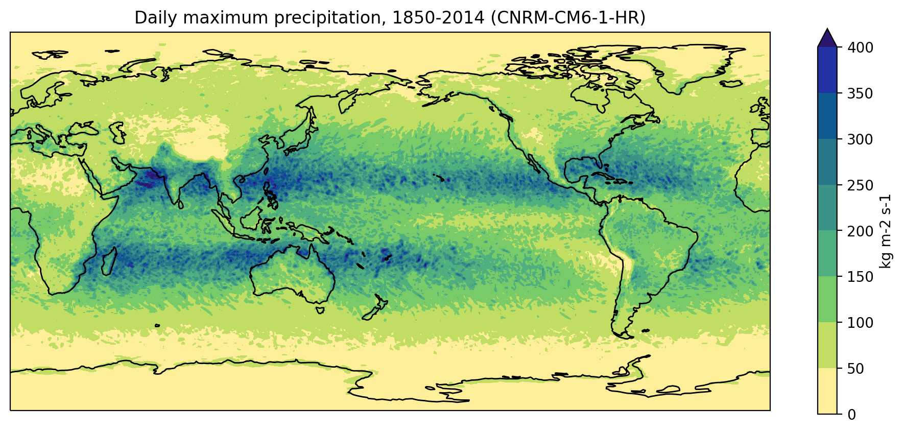
Writing your own Dask-aware functions
So far leveraging Dask for our large data computations has been
relatively simple, because almost all of xarray’s built-in
operations (like max) work on Dask arrays.
If we wanted to chunk and parallelise code involving operations that
aren’t built into xarray (e.g. an interpolation routine
from the SciPy library) we’d first need to use the
apply_ufunc or map_blocks function to make
those operations “Dask-aware”. There’s an xarray
tutorial that explains how to do this.
Alternatives to Dask
While dask can be a good option for working with large
data, it’s not always the best choice. For instance, in this lesson
we’ve talked about the time cost associated with setting up and
coordinating jobs across multiple cores, and the fact that it can take a
bit of time and effort to make a function Dask-aware.
What other options/tactics do you have when working with a large, multi-file dataset? What are the pros and cons of these options?
Other options include writing a loop to process each netCDF file one at a time or a series of sub-regions one at a time.
By breaking the data processing down like this you might avoid the need to make your function/s Dask-aware. If the loop only involves tens (as opposed to hundreds) files/regions, the loop might also not be too slow. However, using Dask is neater and more scalable, because the code you write looks essentially the same regardless of whether you’re running the code on a powerful supercomputer or a personal laptop.
Find out what you’re working with
Setup a Dask client in your Jupyter notebook. How many cores do you have available and how much memory?
Applying this to your own work
In your own research, are there any data processing tasks that could benefit from chunking and/or parallelisation? If so, how would you implement it? What size would your chunks be and along what axis? Are all the operations involved already Dask-aware?
Key Points
- Libraries such as dask and xarray can make loading, processing and visualising netCDF data much easier.
- Dask can speed up processing through parallelism but care may be needed particularly with data chunking.