Data processing and visualisation

Overview

Teaching: 20 min
Exercises: 40 min

Questions

How can I create a quick plot of my CMIP data?

Objectives

Import the xarray library and use the functions it contains.

Convert precipitation units to mm/day.

Calculate and plot the precipitation climatology.

Use the cmocean library to find colormaps designed for ocean science.

As a first step towards making a visual comparison of the ACCESS-CM2 and ACCESS-ESM1-5 historical precipitation climatology, we are going to create a quick plot of the ACCESS-CM2 data.

accesscm2_pr_file = 'data/pr_Amon_ACCESS-CM2_historical_r1i1p1f1_gn_201001-201412.nc'

We will need a number of the libraries introduced in the previous lesson.

import xarray as xr
import cartopy.crs as ccrs
import matplotlib.pyplot as plt
import numpy as np

Since geographic data files can often be very large, when we first open our data file in xarray it simply loads the metadata associated with the file (this is known as “lazy loading”). We can then view summary information about the contents of the file before deciding whether we’d like to load some or all of the data into memory.

dset = xr.open_dataset(accesscm2_pr_file)
print(dset)

<xarray.Dataset>
Dimensions:    (bnds: 2, lat: 144, lon: 192, time: 60)
Coordinates:
  * time       (time) datetime64[ns] 2010-01-16T12:00:00 ... 2014-12-16T12:00:00
  * lon        (lon) float64 0.9375 2.812 4.688 6.562 ... 355.3 357.2 359.1
  * lat        (lat) float64 -89.38 -88.12 -86.88 -85.62 ... 86.88 88.12 89.38
Dimensions without coordinates: bnds
Data variables:
    time_bnds  (time, bnds) datetime64[ns] ...
    lon_bnds   (lon, bnds) float64 ...
    lat_bnds   (lat, bnds) float64 ...
    pr         (time, lat, lon) float32 ...
Attributes:
    CDI:                    Climate Data Interface version 1.9.8 (https://mpi...
    source:                 ACCESS-CM2 (2019): \naerosol: UKCA-GLOMAP-mode\na...
    institution:            CSIRO (Commonwealth Scientific and Industrial Res...
    Conventions:            CF-1.7 CMIP-6.2
    activity_id:            CMIP
    branch_method:          standard
    branch_time_in_child:   0.0
    branch_time_in_parent:  0.0
    creation_date:          2019-11-08T08:26:37Z
    data_specs_version:     01.00.30
    experiment:             all-forcing simulation of the recent past
    experiment_id:          historical
    external_variables:     areacella
    forcing_index:          1
    frequency:              mon
    further_info_url:       https://furtherinfo.es-doc.org/CMIP6.CSIRO-ARCCSS...
    grid:                   native atmosphere N96 grid (144x192 latxlon)
    grid_label:             gn
    initialization_index:   1
    institution_id:         CSIRO-ARCCSS
    mip_era:                CMIP6
    nominal_resolution:     250 km
    notes:                  Exp: CM2-historical; Local ID: bj594; Variable: p...
    parent_activity_id:     CMIP
    parent_experiment_id:   piControl
    parent_mip_era:         CMIP6
    parent_source_id:       ACCESS-CM2
    parent_time_units:      days since 0950-01-01
    parent_variant_label:   r1i1p1f1
    physics_index:          1
    product:                model-output
    realization_index:      1
    realm:                  atmos
    run_variant:            forcing: GHG, Oz, SA, Sl, Vl, BC, OC, (GHG = CO2,...
    source_id:              ACCESS-CM2
    source_type:            AOGCM
    sub_experiment:         none
    sub_experiment_id:      none
    table_id:               Amon
    table_info:             Creation Date:(30 April 2019) MD5:e14f55f257cceaf...
    title:                  ACCESS-CM2 output prepared for CMIP6
    variable_id:            pr
    variant_label:          r1i1p1f1
    version:                v20191108
    cmor_version:           3.4.0
    tracking_id:            hdl:21.14100/b4dd0f13-6073-4d10-b4e6-7d7a4401e37d
    license:                CMIP6 model data produced by CSIRO is licensed un...
    CDO:                    Climate Data Operators version 1.9.8 (https://mpi...
    history:                Tue Jan 12 14:50:25 2021: ncatted -O -a history,p...
    NCO:                    netCDF Operators version 4.9.2 (Homepage = http:/...

We can see that our dset object is an xarray.Dataset, which when printed shows all the metadata associated with our netCDF data file.

In this case, we are interested in the precipitation variable contained within that xarray Dataset:

print(dset['pr'])

<xarray.DataArray 'pr' (time: 60, lat: 144, lon: 192)>
[1658880 values with dtype=float32]
Coordinates:
  * time     (time) datetime64[ns] 2010-01-16T12:00:00 ... 2014-12-16T12:00:00
  * lon      (lon) float64 0.9375 2.812 4.688 6.562 ... 353.4 355.3 357.2 359.1
  * lat      (lat) float64 -89.38 -88.12 -86.88 -85.62 ... 86.88 88.12 89.38
Attributes:
    standard_name:  precipitation_flux
    long_name:      Precipitation
    units:          kg m-2 s-1
    comment:        includes both liquid and solid phases
    cell_methods:   area: time: mean
    cell_measures:  area: areacella

We can actually use either the dset['pr'] or dset.pr syntax to access the precipitation xarray.DataArray.

To calculate the precipitation climatology, we can make use of the fact that xarray DataArrays have built in functionality for averaging over their dimensions.

clim = dset['pr'].mean('time', keep_attrs=True)
print(clim)

<xarray.DataArray 'pr' (lat: 144, lon: 192)>
array([[1.8461452e-06, 1.9054805e-06, 1.9228980e-06, ..., 1.9869783e-06,
        2.0026005e-06, 1.9683730e-06],
       [1.9064508e-06, 1.9021350e-06, 1.8931637e-06, ..., 1.9433096e-06,
        1.9182237e-06, 1.9072245e-06],
       [2.1003202e-06, 2.0477617e-06, 2.0348527e-06, ..., 2.2391034e-06,
        2.1970161e-06, 2.1641599e-06],
       ...,
       [7.5109556e-06, 7.4777777e-06, 7.4689174e-06, ..., 7.3359679e-06,
        7.3987890e-06, 7.3978440e-06],
       [7.1837171e-06, 7.1722038e-06, 7.1926393e-06, ..., 7.1552149e-06,
        7.1576678e-06, 7.1592167e-06],
       [7.0353467e-06, 7.0403985e-06, 7.0326828e-06, ..., 7.0392648e-06,
        7.0387587e-06, 7.0304386e-06]], dtype=float32)
Coordinates:
  * lon      (lon) float64 0.9375 2.812 4.688 6.562 ... 353.4 355.3 357.2 359.1
  * lat      (lat) float64 -89.38 -88.12 -86.88 -85.62 ... 86.88 88.12 89.38
Attributes:
    standard_name:  precipitation_flux
    long_name:      Precipitation
    units:          kg m-2 s-1
    comment:        includes both liquid and solid phases
    cell_methods:   area: time: mean
    cell_measures:  area: areacella

Now that we’ve calculated the climatology, we want to convert the units from kg m-2 s-1 to something that we are a little more familiar with like mm day-1.

To do this, consider that 1 kg of rain water spread over 1 m2 of surface is 1 mm in thickness and that there are 86400 seconds in one day. Therefore, 1 kg m-2 s-1 = 86400 mm day-1.

The data associated with our xarray DataArray is simply a numpy array,

type(clim.data)

numpy.ndarray

so we can go ahead and multiply that array by 86400 and update the units attribute accordingly:

clim.data = clim.data * 86400
clim.attrs['units'] = 'mm/day' 

print(clim)

<xarray.DataArray 'pr' (lat: 144, lon: 192)>
array([[0.15950695, 0.16463352, 0.16613839, ..., 0.17167493, 0.17302468,
        0.17006743],
       [0.16471735, 0.16434446, 0.16356934, ..., 0.16790195, 0.16573453,
        0.1647842 ],
       [0.18146767, 0.17692661, 0.17581128, ..., 0.19345854, 0.18982219,
        0.18698342],
       ...,
       [0.64894656, 0.64607999, 0.64531446, ..., 0.63382763, 0.63925537,
        0.63917372],
       [0.62067316, 0.61967841, 0.62144403, ..., 0.61821057, 0.6184225 ,
        0.61855632],
       [0.60785395, 0.60829043, 0.60762379, ..., 0.60819248, 0.60814875,
        0.6074299 ]])
Coordinates:
  * lon      (lon) float64 0.9375 2.812 4.688 6.562 ... 353.4 355.3 357.2 359.1
  * lat      (lat) float64 -89.38 -88.12 -86.88 -85.62 ... 86.88 88.12 89.38
Attributes:
    standard_name:  precipitation_flux
    long_name:      Precipitation
    units:          mm/day
    comment:        includes both liquid and solid phases
    cell_methods:   area: time: mean
    cell_measures:  area: areacella

We could now go ahead and plot our climatology using matplotlib, but it would take many lines of code to extract all the latitude and longitude information and to setup all the plot characteristics. Recognising this burden, the xarray developers have built on top of matplotlib.pyplot to make the visualisation of xarray DataArrays much easier.

fig = plt.figure(figsize=[12,5])

ax = fig.add_subplot(111, projection=ccrs.PlateCarree(central_longitude=180))

clim.plot.contourf(ax=ax,
                   levels=np.arange(0, 13.5, 1.5),
                   extend='max',
                   transform=ccrs.PlateCarree(),
                   cbar_kwargs={'label': clim.units})
ax.coastlines()

plt.show()

Precipitation climatology

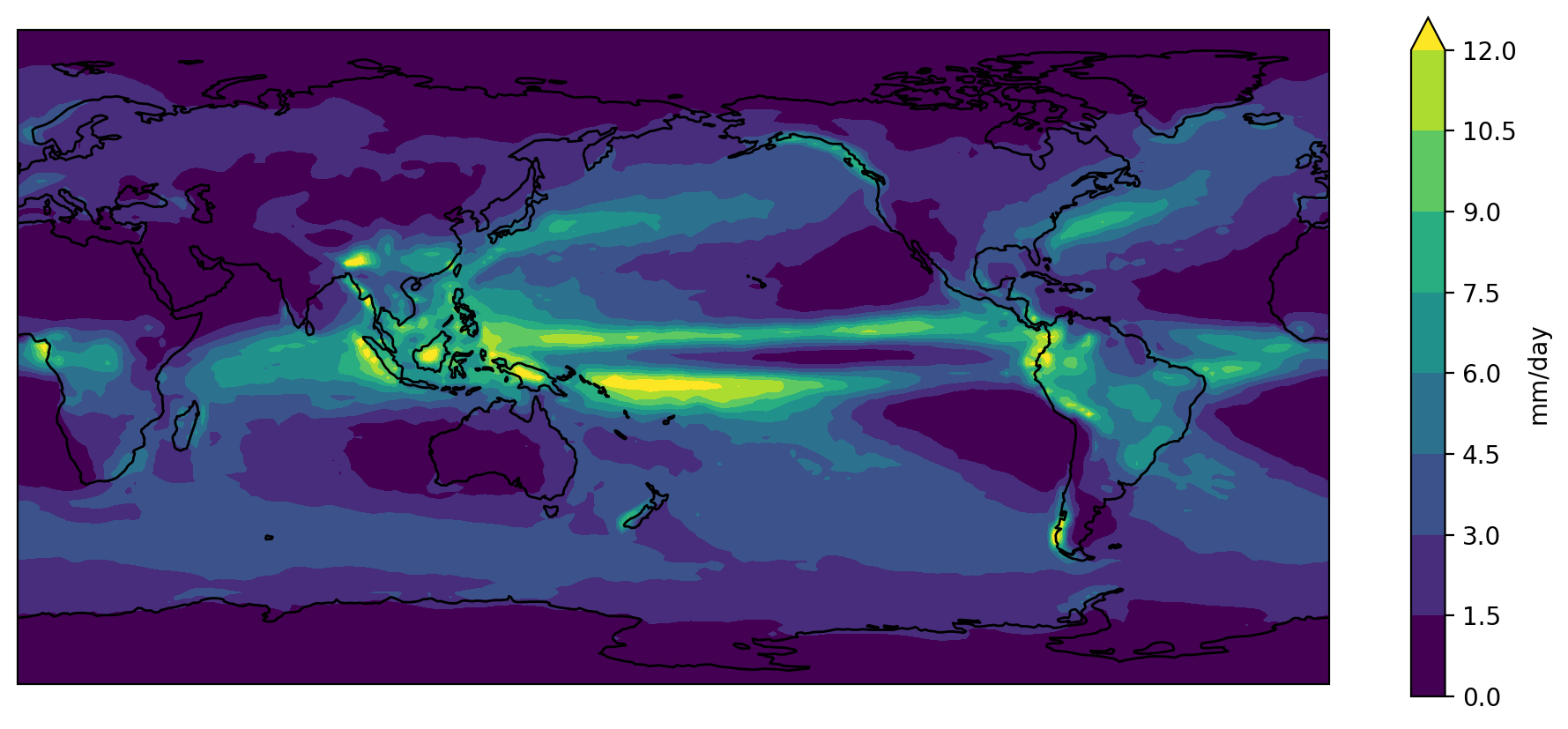
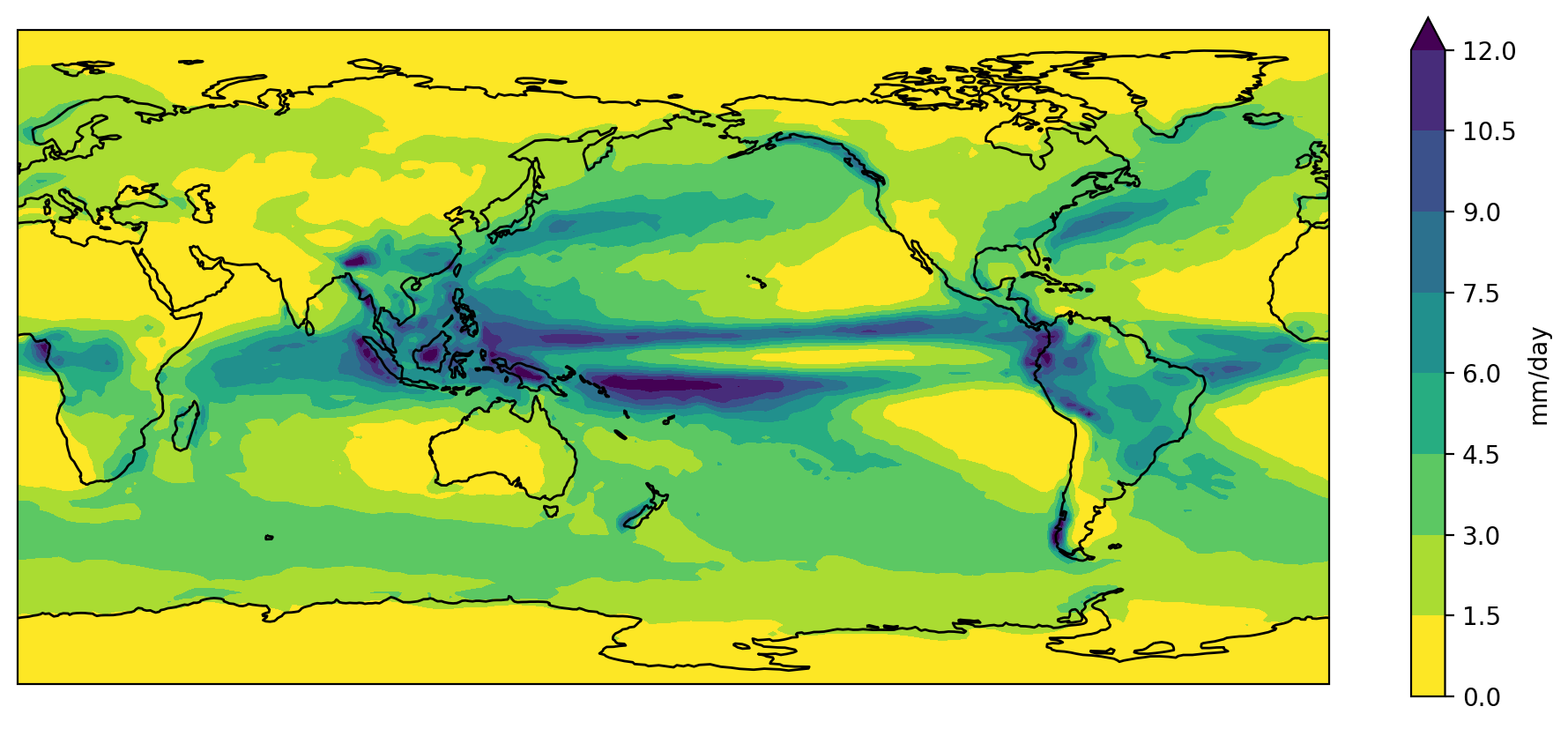
The default colorbar used by matplotlib is viridis. It used to be jet, but that was changed a couple of years ago in response to the #endtherainbow campaign.

Putting all the code together (and reversing viridis so that wet is purple and dry is yellow)…

import xarray as xr
import cartopy.crs as ccrs
import matplotlib.pyplot as plt
import numpy as np

accesscm2_pr_file = 'data/pr_Amon_ACCESS-CM2_historical_r1i1p1f1_gn_201001-201412.nc'

dset = xr.open_dataset(accesscm2_pr_file)

clim = dset['pr'].mean('time', keep_attrs=True)

clim.data = clim.data * 86400
clim.attrs['units'] = 'mm/day'

fig = plt.figure(figsize=[12,5])
ax = fig.add_subplot(111, projection=ccrs.PlateCarree(central_longitude=180))
clim.plot.contourf(ax=ax,
                   levels=np.arange(0, 13.5, 1.5),
                   extend='max',
                   transform=ccrs.PlateCarree(),
                   cbar_kwargs={'label': clim.units},
                   cmap='viridis_r')
ax.coastlines()
plt.show()

Precipitation climatology

Color palette

Copy and paste the final slab of code above into your own Jupyter notebook.

The viridis color palette doesn’t seem quite right for rainfall. Change it to the “haline” cmocean palette used for ocean salinity data.
Solution
import cmocean

...
clim.plot.contourf(ax=ax,
                       ...
                       cmap=cmocean.cm.haline_r)

Season selection

Rather than plot the annual climatology, edit the code so that it plots the June-August (JJA) season.

(Hint: the groupby functionality can be used to group all the data into seasons prior to averaging over the time axis)
Solution
clim = dset['pr'].groupby('time.season').mean('time', keep_attrs=True) 
clim.data = clim.data * 86400
clim.attrs['units'] = 'mm/day'

clim.sel(season='JJA').plot.contourf(ax=ax,
                                     ...

Add a title

Add a title to the plot which gives the name of the model (taken from the dset attributes) followed by the words “precipitation climatology (JJA)”
Solution
model = dset.attrs['source_id']
title = f'{model} precipitation climatology (JJA)'
plt.title(title)

Key Points

Libraries such as xarray can make loading, processing and visualising netCDF data much easier.

The cmocean library contains colormaps custom made for the ocean sciences.

previous episode

Python for Atmosphere and Ocean Scientists

next episode

Data processing and visualisation

Overview

Color palette

Solution

Season selection

Solution

Add a title

Solution

Key Points

previous episode

next episode