First Steps on R
Overview
Teaching: 10 min
Exercises: 10 minQuestions
What is R, and why is important to learn to use it?
What types of data does the R language has?
Objectives
Understand why R is important.
Describe the purpose and use of each panel in the RStudio IDE
Locate buttons and options in the RStudio IDE
Define a variable
Assign data to a variable
It takes courage to sail in uncharted waters -Snoopy
RStudio setup
What is R, and what can it be used for?
“R” is used to name a programming language and the software that reads and interprets the instructions written on the scripts of this language. Is specialized in statistical computing and graphics. RStudio is the most popular program for script writing and interaction with R software.
R uses a series of written commands, which is great, believe us! If you rely on clicking, pointing, and remembering where and why to point here or click there, mistakes are prone to occur. Moreover, if you manage to get more data, it is easier to just re-run your script to obtain results. Also, working with scripts makes the steps you follow for your analysis clear and shareable. Here are some of the advantages of working with R:
- R code is reproducible
- R produces high-quality graphics
- R has a large community
- R is interdisciplinary
- R works on data of all colors and sizes
- R is free!
A nautical chart of RStudio
RStudio is an Integrated Development Environment(IDE) which we will use to write code, navigate the files from our computer/cloud, try code, inspect the variables we are going to create, and visualize our plots.
Here is what you may look at the first time you open RStudio:
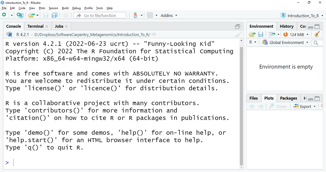
The figure shows the RStudio interface. The three windows that appear on the screen provide us with a space in which we can see our console (left side window) where the orders we want to execute are written, observe the generated variables (upper right), and a series of subtabs (lower right): Files shows us files that we have used, Plots shows us graphics that we are generating, Packages shows the packages that we have downloaded, Help it gives us information on packages, commands, and/or functions that we do not know, but works only with an internet connection, and Viewer shows a results preview in R markdown files.
If we click on the option File/New File/R Script, we open up a script and
we get what we can call an RStudio nautical chart
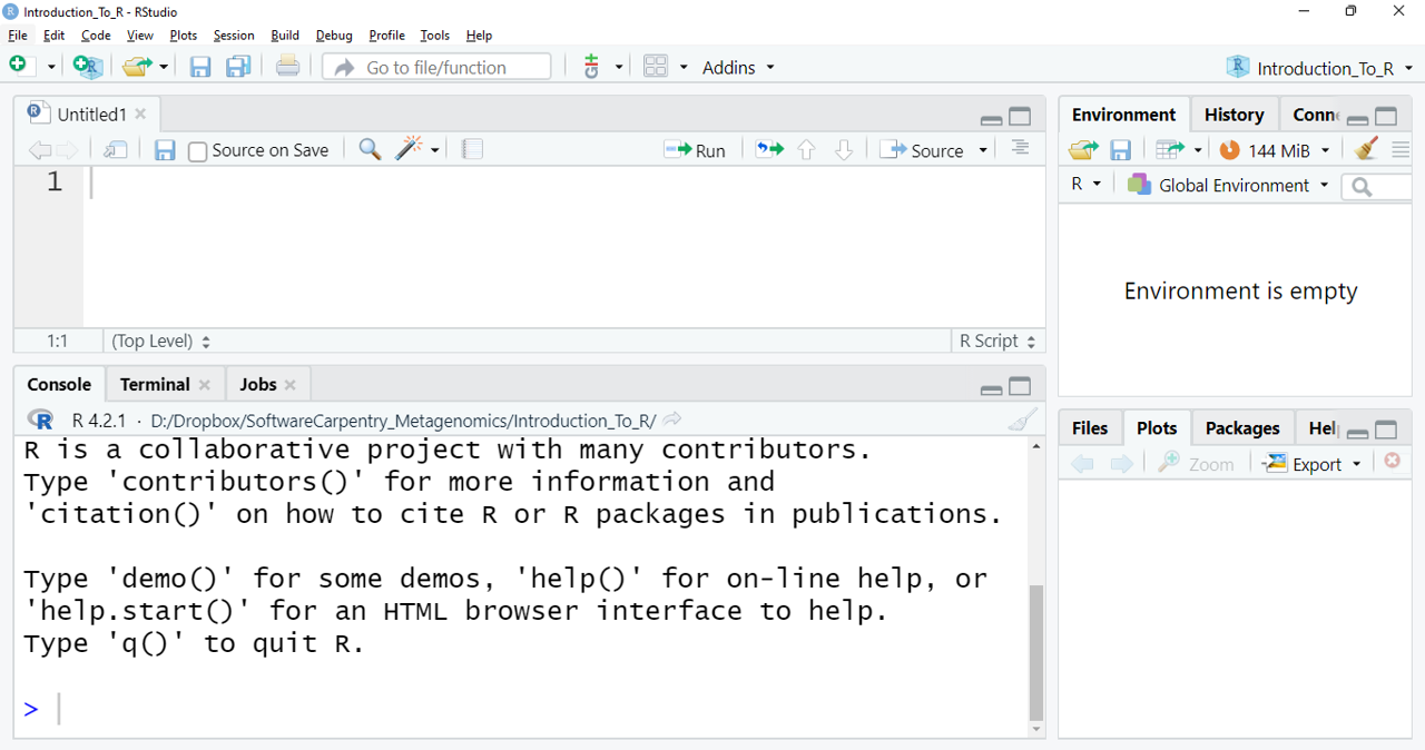
RStudio interface with a new panel is shown. Clockwise from top left: Empty script,
Environment/History/Connections/Tutorial, Files/Plots/Packages/Help/Viewer,
Console/Terminal/Jobs. You can enter your online RStudio to see your environment.
Let’s copy your instance address into your browser (Chrome or Firefox) and login into Rstudio.
The address should look like this: http://ec2-3-235-238-92.compute-1.amazonaws.com:8787/ Although
data are already stored in your instance, in case you need to you can download them here.
Review of the setup
As we have revisited throughout the lesson, maintaining related data in a single folder
is desirable. In RStudio, this folder is called the working directory. It is where R will be looking
for and saving your files. If you need to check where your working directory is located use getwd().
If your working directory is not what you expected(i.e. ~/dc_workshop/taxonomy/), it can always be changed by clicking on the blue
gear icon:
 on the
 Files tab, pick the option Set As Working Directory. Alternatively, you can use the setwd() command for changing it.
Let’s use these commands to set our working directory where we have stored our files from the previous lessons:
> setwd("~/dc_workshop/taxonomy/")
Having a dialogue with R
There are two main paths to interact with R in RStudio:
- Using the console.
- Creating and editing script files.
The console is where commands can be typed and executed immediately, and where the
results from executed commands will be displayed (like in the Unix shell). If R is ready to accept commands, the R console shows
the > prompt. You can type instructions directly into the console and press “Enter”, but they will
be forgotten when you close the session.
For example, let’s do some math and save it in R objects. We can store values in variables by
using the assignment operator <-:
> 4+3
> addition <- 4+3
> subtraction <- 2+1
> total <- addition -subtraction
> total
What would happen if you tap ctrl + l? Without the lesson page, can you remember what numbers the sum is made of in the variable addition?
Reproducibility is in our minds when we program (and when we do science). For this purpose,
is convenient to type the commands we want to save in the script editor, and save the script periodically.
We can run our code lines in the script by the shortcut ctrl + Enter
(on Mac, Cmd + Return will work). Thus, the command on the current line or the instructions
in the currently selected text will be sent to the console and will be executed.
Time can be the enemy or ally of memory. We want to be sure to remember why we wrote the commands
in our scripts, so we can leave comments(lines of no executable text) by beginning a line with #:
# Let's do some math in RStudio. How many times a year do the supermarkets change the bread that they use for
# display? if they change it every 15 days:
> 365/15
[1] 24.3333
Key Points
R is a programming language
RStudio is a useful tool for script writing and data-management.
A variable can temporarily store data.
R Data Types
Overview
Teaching: 10 min
Exercises: 5 minQuestions
What types of data does the R language have?
Objectives
Learn the types of data that we can manage in R.
Types of data
We already used numbers to generate a result. But this is not the only type of data that RStudio
can manage. We can use the command typeof() to corroborate the data type of our object addition:
> typeof(addition)
> [1] "double"
There are five types of data in RStudio:
- Double
- Integer
- Complex
- Logical
- Character
> typeof(5L) #Integer type can contain only whole numbers followed by a capital L
[1] "integer"
> typeof(72+5i)
[1] "complex"
> addition == subtraction
[1] FALSE
> typeof(addition == subtraction)
[1] "logical"
> result <- "4 and 3 are not the same on Earth. On Mars maybe... "
> typeof(result)
[1] "character"
No matter how complicated our analysis can be, all data in R will belong to one of these five data types. Data types are important because we want to know “who is who, and what is what”. But this concept will help us learn one of the most powerful tools in R, which is the manipulation of diverse types of data together in what is called a data-frame.
Data structures
Besides the data types, there are different ways of organizing the data in R called data structures. The simple data structure is the vector, which is a sequence of data of the same type. We can create a vector with the function c().
> char_vector <- c("a", "a", "b", "b", "c", "c")
> typeof(char_vector)
[1] "character"
A more complex data structure is the factor, which holds the names of categories (called levels) and a sequence of the occurrences of those categories. Here we can see how factor works:
> char_factor <- as.factor(char_vector)
> char_factor
[1] a a b b c c
Levels: a b c
And here, we can ask for the structure of the object.
> str(char_factor)
Factor w/ 3 levels "a","b","c": 1 1 2 2 3 3
Here, you see the levels of the factors and a sequence of numbers. Each number represents a level, and this sequence holds the information about which goes in which position. That is why we will get an “integer” if we ask about the type of data in the object.
> typeof(char_factor)
[1] "integer"
When we are dealing with categorical data, factors are the way to go.
Exercise 1: Types and structures of data
Which type of data is present in each of the next vectors?:
ej1 <- c("34","147","26+7i")
ej2 <- c(4L,12L,152L)
ej3 <- c(34,147,26+7i)A) numerical, integer, numerical
B) character, numerical, numerical
C) numerical, complex, character
D) character, integer, complex
がんばって! (ganbatte; good luck):
Solution
The correct answer is: D) character, integer, complex.
If we use
""to define an object, R will read it as a character regardless we are typing numbers.
The capitalLafter a number, indicates R to save that number as an Integer.
And each set of numbers with the letteriof imaginary, indicates R that this is a set of complex numbers.
Key Points
R uses different types of data to store information.
Data Frame Manipulation
Overview
Teaching: 10 min
Exercises: 10 minQuestions
Data-frames. What are they, and how to manage them?
Objectives
Understand what is a data-frame and learn to manipulate it.
Data-frames: The power of interdisciplinarity
Data-frames are the powerful data structures in R. Let’s begin by creating a mock data set:
> musician <- data.frame(people = c("Medtner", "Radwimps", "Shakira"),
						 pieces = c(722,187,68),
 						 likes = c(0,1,1))
> musician
The content of our new object:
    people pieces likes
1  Medtner    722     0
2 Radwimps    187     1
3  Shakira     68     1
We have just created our first data-frame. We can see if this is true using the class() command:
> class(musician)
[1] "data.frame"
A data-frame is a collection of vectors (i.e. a list) whose components must be of the same data type within each vector:
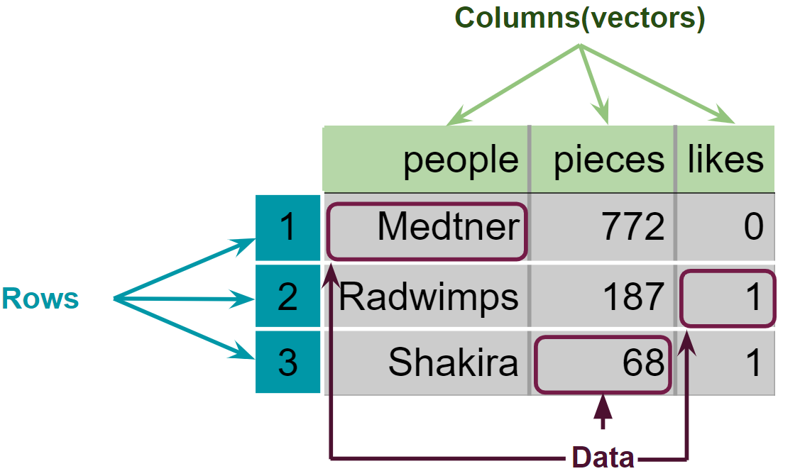 Figure 3. Structure of the created data-frame.
We can begin to explore our new object by pulling out columns using the $ operator. In order to use it,
you need to write the name of your data-frame, followed by the $ operator and the name of the column
you want to extract:
> musician$people
[1] "Medtner" "Radwimps" "Shakira"
We can do operations with the columns:
> musician$pieces + 20
[1] 742 207 88
Moreover, we can change the data type of one of the columns. Using the next line of code we can see if the musicians are popular or not:
> typeof(musician$likes)
[1] "double"
> musician$likes <- as.logical(musician$likes)
> paste("Is",musician$people, "popular? :", musician$likes, sep = " ")
[1] "Is Medtner popular? : FALSE" "Is Radwimps popular? : TRUE" "Is Shakira popular? : TRUE"
Finally, we can extract information from a specific place in our data by using the “matrix” nomenclature [-,-],
where the first number inside the brackets specifies the row number, and the second the column number:
![Dataframe shown as table, showing that [1,] corrseponds to row 1, [2,] to row two, [3,] to row 3, [,1] to clumn 1, [,2] to column 2, [,3] to column 3. And pinting to location [1,2] that corresponds to the number 772](https://user-images.githubusercontent.com/67386612/119908857-2a517080-bf19-11eb-8e0f-b3da6d1dcfc0.png) Figure 4. Extraction of specific data in a data-frame and a matrix.
Figure 4. Extraction of specific data in a data-frame and a matrix.
> musician[1,2] # The number of pieces that Nikolai Medtner composed
[1] 722
We can also call for that data by calling the column by it’s name
> musician[1,"pieces"] # The number of pieces that Nikolai Medtner composed
[1] 722
Exercise 2:
Complete the lines of code to obtain the required information
Code Information required > musician[__,__] Pieces composed by Shakira > (musician____)_2 Pieces composed by all musicians if they were half of productive (The half of their actual pieces) > musician$___ <- c(,,___) Redefine the likescolumn to make all the musicians popular!がんばって! (ganbatte; good luck):
Solution
Code Information required > musician[3,”pieces”] Pieces composed by Shakira > (musician$pieces)/2 Pieces composed by all musicians if they were half of productive (The half of their actual pieces) > musician$likes <- c(“TRUE”,”TRUE”,”TRUE”) Redefine the likescolumne to make all the musicians popular!
Key Points
Data-frames contain multiple columns with different types of data.
Making Graphs with ggplot2
Overview
Teaching: 15 min
Exercises: 10 minQuestions
How can I create useful graphs in R?
Objectives
Create figures using ggplot2.
Install and use libraries in R.
R Libraries
Until now, we have used the basal functions included in the R language. But, R can use groups of functions for diverse purposes. These are called packages or libraries. A package is a family of code units (functions, classes, variables) that implement a set of related tasks. Installing a package is like buying a new piece of lab equipment. Loading a package is like getting that piece of lab equipment out of a storage locker and setting it up in the working space. Packages provide additional functionality to the basic R code, much like a new piece of equipment adds functionality to a lab space. R has its own base plotting system, but we will use a package that will help us to create more artistic figures:ggplot2.
Let’s install the ggplot2 library.
> install.packages("ggplot2")
Now that it is installed we have to load it. It is a good practice to load all the libraries that you will use in a script at the beginning of that script.
library(ggplot2)
Visualizing data with ggplot2
ggplot2 has been created with the idea that any graph can be expressed with three components:
- Data set
- Coordinates
- Set of geoms, that is the visual representation of the data
These geoms can be thought of as layers that can be overlapped one over another, so special care is required to show useful information layers to deliver a message. We are going to create an example with some of the data that we already have.
> musician
    people pieces likes
1  Medtner    722 FALSE
2 Radwimps    187  TRUE
3  Shakira     68  TRUE
First, let’s try to make a figure only with the data and coordinates components, to see what we are talking about.
> ggplot(data= musician,
       mapping = aes(x = people, y = pieces))
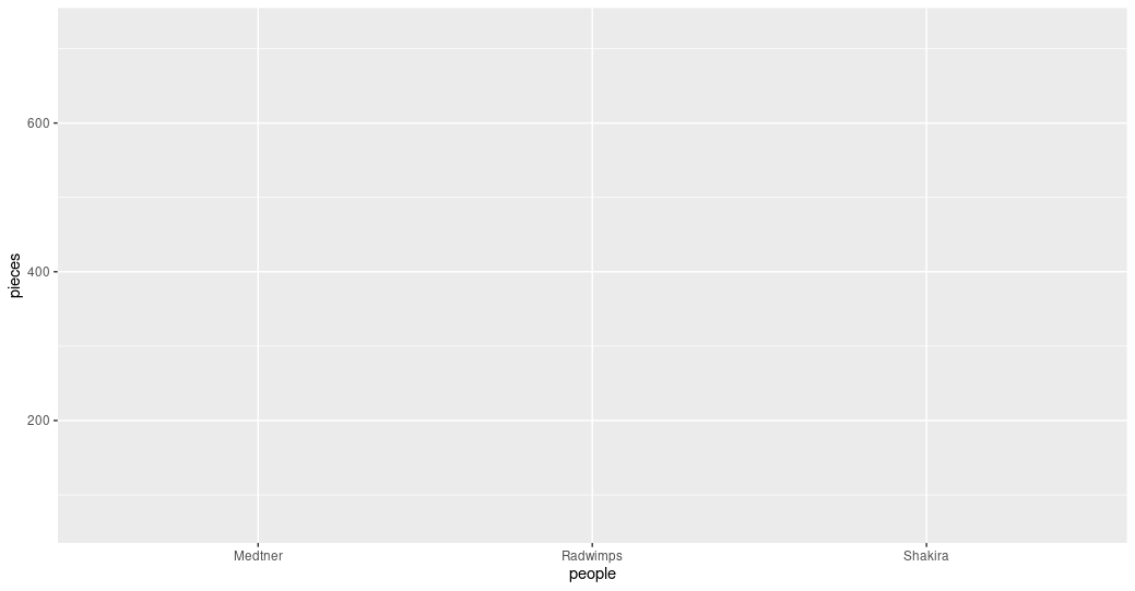 Figure 1. A graph without data representation.
Unraveling the above code. We first called the ggplot function (i.e. ggplot()). This will tell R that we want to
create a new plot, and the parameters indicated inside this function will apply to all the layers of the plot. We
gave two arguments to the ggplot code: (i) the data that we want to show in our figure (i.e. data = musician),
and (ii) the way of displaying it in the graph (i.e. mapping = aes(x = people,y = pieces)),
which will tell ggplot how the variables will be mapped in the figure. In this case, x is the name of the
musicians, and y is the number of pieces each of them composed. It is noticeable that we did not need to express the entire path to access
these columns to the aes function (i.e. x = musician[,”people”]). That is because the code is so well
written that figures it out by itself. With this, we have made the base of our plot, but we can’t see the data
because we have not chosen a graphic way of representing it (i.e. the geoms).
> ggplot(data= musician,
        mapping = aes(x = people, y = pieces))+
  geom_col()
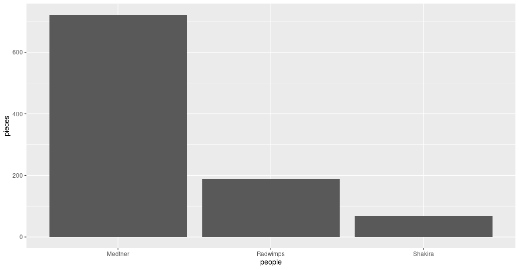 Figure 2. Bar plot of the pieces composed by each musician.
Some elements of the graphs can be informative or merely decorative. If we want it to be informative, it needs to go
inside the aes() function and say what information it will display. If we want it to be decorative it must be outside of aes().
Let’s see how this work with the color.
> ggplot(data= musician,
       mapping = aes(x = people, y = pieces))+
  geom_col(color = "blue")
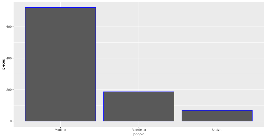 Figure 3. Bar plot with the decorative color parameter.
ggplot(data= musician,
       mapping = aes(x = people, y = pieces))+
  geom_col(aes(color= likes))
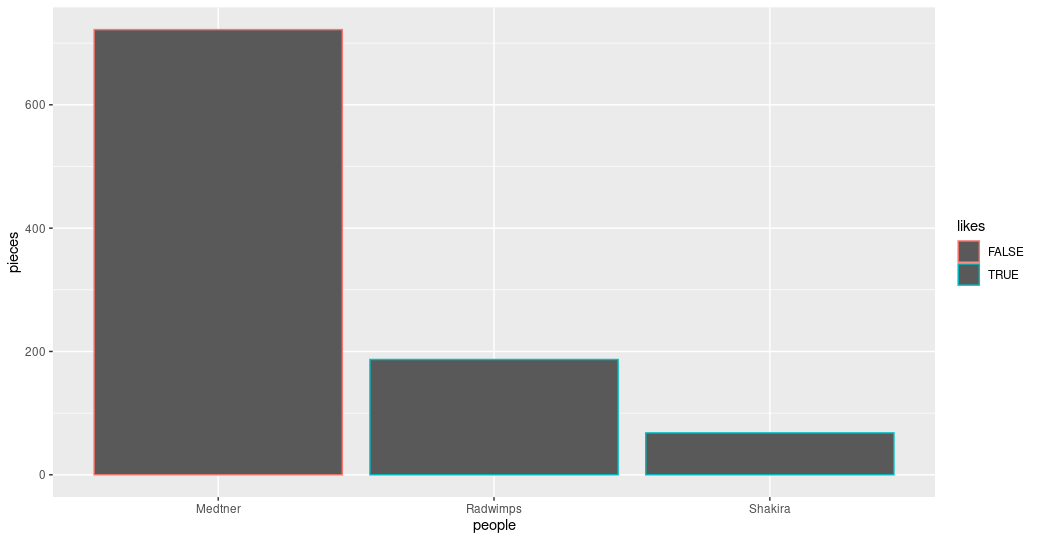 Figure 4. Bar plot with the informative color parameter.
Exercise 1: Global and specific parameters.
Search for more available geoms and chose one that is appropriate to display the same information as the bars. Add it to your graph using the
+sign after the last geom. Explore what happens if the color parameters are in theggplot()part of the command or in each of the geoms.Solution
ggplot(data= musician,
      mapping = aes(x = people, y = pieces))+
 geom_col(aes(color= likes))+
 geom_point()
Figure 5. Bar and point plot.
ggplot(data= musician,
      mapping = aes(x = people, y = pieces, color= likes))+
 geom_col()+
 geom_point()
Figure 6. Bar and point plot with global color.
Advanced exercise: Personalize informative colors.
Search how to personalize which colors are used when the color is an informative parameter.
Solution
ggplot(data= musician,
      mapping = aes(x = people, y = pieces, color= likes))+
 scale_color_manual(values= c("blue", "orange"))+
 geom_col()+
 geom_point()
Figure 7. Bar and point plot with personalized colors.
Key Points
The library
ggplot2creates plots that help/remarks the data analysis.Creativity is welcome to explore and present your data.
Libraries in R allow us to have sets of functions specialized in a global purpose.
Finding Help on R
Overview
Teaching: 5 min
Exercises: 0 minQuestions
How can I ask R for help?
Objectives
Use the help command to get more insight on R functions.
Seeking help
If you face some trouble with some function, let’s say summary(), you can always type ?summary()
and a help page will be displayed with useful information regarding that function. Furthermore, if you
already know what you want to do, but you do not know which function to use, you can type ??
following your inquiry, for example ??barplot will open a help file in the RStudio’s help
panel in the lower right corner.
With this, we have the needed tools to begin our exploration of diversity with R. That does not mean that we have already covered all that R have to offer, if you want to know more about R, we recommend you to check the R lesson for Reproducible genomic analysis. Let’s continue and see what this journey has to offer.
Key Points
Help
?shows useful information about the functions you inquire.